Filling Undefined Values

When working with gridded data, undefined values (NaNs) can be problematic for interpolation, especially near land/sea masks. If any of the grid points used for interpolation are undefined, the result will also be undefined. This example demonstrates multiple methods to fill these undefined values and provides guidance on choosing the best method for your use case.

The Problem with Undefined Values

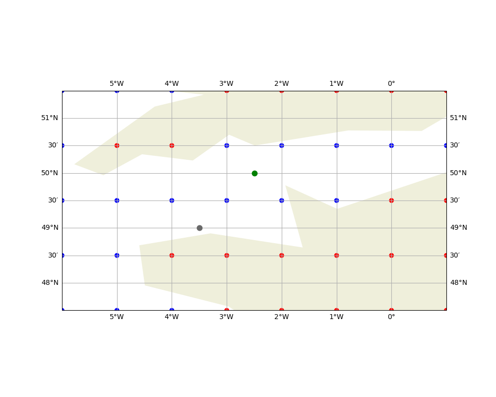
To illustrate the issue, consider the following grid where some values are undefined (represented by red points). If we want to interpolate the value at the gray point using bilinear interpolation, the calculation will fail because one of the surrounding grid points is undefined. However, the green point can be interpolated without any issues because all its surrounding points are defined.

import time

import cartopy.crs
import cartopy.feature
import matplotlib.pyplot
import numpy

import pyinterp.backends.xarray
import pyinterp.fill
import pyinterp.tests

fig = matplotlib.pyplot.figure(figsize=(10, 8))
ax = fig.add_subplot(111, projection=cartopy.crs.PlateCarree())
ax.set_extent([-6, 1, 47.5, 51.5], crs=cartopy.crs.PlateCarree())
ax.add_feature(cartopy.feature.LAND.with_scale('110m'))
ax.gridlines(draw_labels=True, dms=True, x_inline=False, y_inline=False)

lons, lats = numpy.meshgrid(numpy.arange(-6, 2),
                            numpy.arange(47.5, 52.5),
                            indexing='ij')
mask = numpy.array([
    [1, 1, 1, 0, 0, 0, 0, 0],  # yapf: disable
    [1, 1, 0, 0, 0, 0, 0, 0],  # yapf: disable
    [1, 1, 1, 1, 1, 1, 0, 0],  # yapf: disable
    [1, 0, 0, 1, 1, 1, 1, 1],  # yapf: disable
    [1, 1, 1, 0, 0, 0, 0, 0]
]).T
ax.scatter(lons.ravel(),
           lats.ravel(),
           c=mask,
           cmap='bwr_r',
           transform=cartopy.crs.PlateCarree(),
           vmin=0,
           vmax=1)
ax.plot([-3.5], [49], linestyle='', marker='.', color='dimgray', markersize=15)
ax.plot([-2.5], [50], linestyle='', marker='.', color='green', markersize=15)
fig.show()

Note

This issue does not affect nearest-neighbor interpolation, as it does not perform any arithmetic operations on the grid values.

Filling with LOESS (Local Regression)

The pyinterp.fill.loess() function uses a fundamentally different approach from the other methods. Instead of solving a partial differential equation, it performs weighted local polynomial regression using a tri-cube weight function: \(w(x)=(1-|d|^3)^3\).

When to use LOESS:

• You want to smooth noisy data while filling gaps

• You need local control over the filling process

• The gaps are small relative to the defined regions

• You want to filter or extrapolate boundary values

Limitations:

• Does not guarantee smooth harmonic fills

• Window size (nx, ny) must be tuned to your data

• Can be slower for large grids

Let’s demonstrate with real data:

ds = pyinterp.tests.load_grid2d()
grid = pyinterp.backends.xarray.Grid2D(ds.mss)

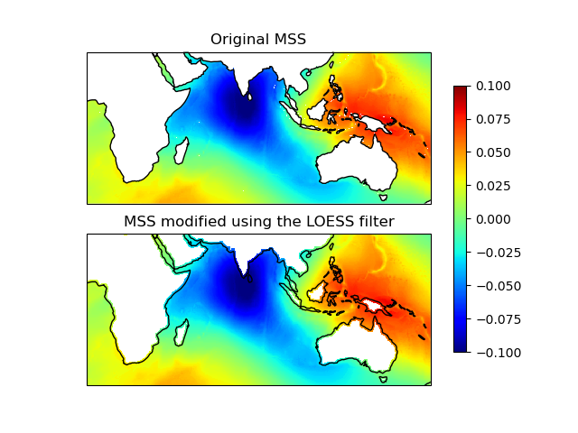
The LOESS method can fill undefined values and also filter defined ones:

filled = pyinterp.fill.loess(grid, nx=3, ny=3)

Let’s visualize the original and filled grids:

fig = matplotlib.pyplot.figure(figsize=(10, 8))
fig.subplots_adjust(left=0.05, right=0.95, top=0.95, bottom=0.05, hspace=0.25)
ax1 = fig.add_subplot(
    211, projection=cartopy.crs.PlateCarree(central_longitude=180))
lons, lats = numpy.meshgrid(grid.x, grid.y, indexing='ij')
pcm = ax1.pcolormesh(lons,
                     lats,
                     ds.mss.T,
                     cmap='jet',
                     shading='auto',
                     transform=cartopy.crs.PlateCarree(),
                     vmin=-0.1,
                     vmax=0.1)
ax1.coastlines()
ax1.set_title('Original MSS')
ax1.set_extent([0, 170, -45, 30], crs=cartopy.crs.PlateCarree())
ax2 = fig.add_subplot(
    212, projection=cartopy.crs.PlateCarree(central_longitude=180))
pcm = ax2.pcolormesh(lons,
                     lats,
                     filled,
                     cmap='jet',
                     shading='auto',
                     transform=cartopy.crs.PlateCarree(),
                     vmin=-0.1,
                     vmax=0.1)
ax2.coastlines()
ax2.set_title('Filled MSS with LOESS (nx=3, ny=3)')
ax2.set_extent([0, 170, -45, 30], crs=cartopy.crs.PlateCarree())
fig.colorbar(pcm, ax=[ax1, ax2], shrink=0.8)

<matplotlib.colorbar.Colorbar object at 0x13e085730>

Comparing PDE-Based Fill Methods

The remaining methods (Gauss-Seidel, Multi-grid, and FFT Inpaint) all solve the Laplace equation to create smooth, harmonic fills. To compare them, let’s create a synthetic test case with a known analytical solution.

We’ll use a 2D Gaussian field with artificial gaps:

# Create a synthetic field
nx, ny = 200, 150
x = numpy.linspace(-5, 5, nx)
y = numpy.linspace(-5, 5, ny)
xx, yy = numpy.meshgrid(x, y, indexing='ij')

# Analytical field: 2D Gaussian
true_field = numpy.exp(-(xx**2 + yy**2) / 4)

# Create gaps (simulate land mask)
mask_gaps = numpy.zeros((nx, ny), dtype=bool)
# Central circular gap
mask_gaps[(xx**2 + yy**2) < 2] = True
# Irregular boundary gaps
mask_gaps[30:50, 40:100] = True
mask_gaps[120:140, 60:90] = True

# Apply mask
field_with_gaps = true_field.copy()
field_with_gaps[mask_gaps] = numpy.nan

Let’s visualize the test field:

fig, axes = matplotlib.pyplot.subplots(1, 2, figsize=(12, 5))
fig.subplots_adjust(wspace=0.3)

im1 = axes[0].imshow(true_field.T,
                     origin='lower',
                     cmap='viridis',
                     aspect='auto')
axes[0].set_title('True Analytical Field (2D Gaussian)')
axes[0].set_xlabel('X')
axes[0].set_ylabel('Y')
fig.colorbar(im1, ax=axes[0])

im2 = axes[1].imshow(field_with_gaps.T,
                     origin='lower',
                     cmap='viridis',
                     aspect='auto')
axes[1].set_title('Field with Gaps (NaN values)')
axes[1].set_xlabel('X')
axes[1].set_ylabel('Y')
fig.colorbar(im2, ax=axes[1])

<matplotlib.colorbar.Colorbar object at 0x13df9ef00>

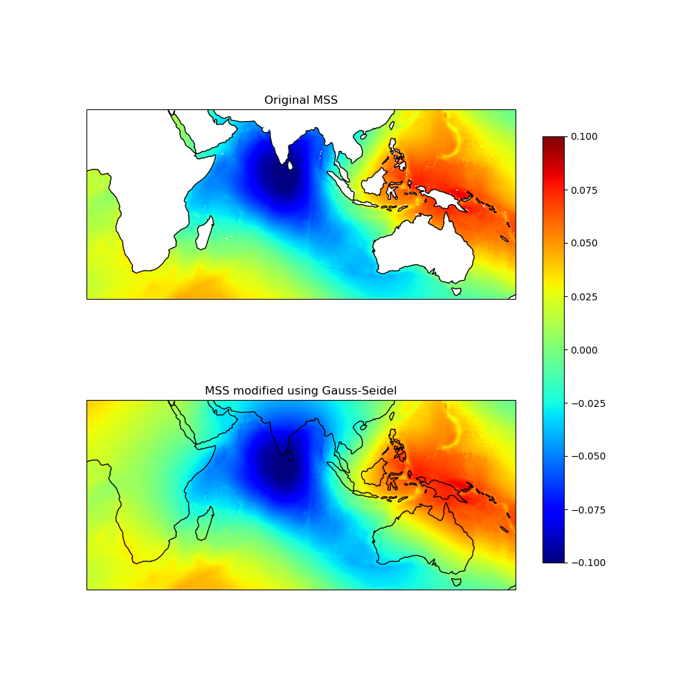
Gauss-Seidel Method

pyinterp.fill.gauss_seidel() uses iterative relaxation to solve the Laplace equation. It’s straightforward and predictable with explicit control over relaxation parameters.

When to use Gauss-Seidel:

• Small to medium-sized grids (< 500×500)

• You need precise control over convergence and relaxation

• Simple, predictable behavior is important

• You’re debugging or validating fill behavior

start = time.time()
iterations_gs, residual_gs, filled_gs = pyinterp.fill.gauss_seidel(
    field_with_gaps.astype(numpy.float64),
    is_circle=False,
    epsilon=1e-4,
)
time_gs = time.time() - start

print(f'Gauss-Seidel: {iterations_gs} iterations, '
      f'residual={residual_gs:.2e}, time={time_gs:.3f}s')

Gauss-Seidel: 225 iterations, residual=9.92e-05, time=0.036s

Multi-grid Method

pyinterp.fill.multi_grid() uses a V-cycle approach that solves the problem at multiple resolution levels. It’s generally the fastest method for large grids.

When to use Multi-grid:

• Large grids (> 500×500)

• You need the fastest possible solution

• Convergence speed is critical

• Production pipelines processing many grids

Advantages over Gauss-Seidel:

• Typically 2-10× faster for large grids

• Better convergence properties

• More efficient memory access patterns

start = time.time()
iterations_mg, residual_mg, filled_mg = pyinterp.fill.multi_grid(
    field_with_gaps.astype(numpy.float64),
    is_circle=False,
    epsilon=1e-4,
)
time_mg = time.time() - start

print(f'Multi-grid: {iterations_mg} iterations, '
      f'residual={residual_mg:.2e}, time={time_mg:.3f}s')

Multi-grid: 119 iterations, residual=9.78e-05, time=0.910s

FFT Inpaint Method

pyinterp.fill.fft_inpaint() uses spectral methods (FFT or DCT) with a Gaussian low-pass filter to create smooth fills.

When to use FFT Inpaint:

• You want very smooth, spectrally-controlled fills

• The grid has periodic or reflective boundaries

• You need to control smoothness via the sigma parameter

• Spectral properties of the fill matter

Trade-offs:

• Can be faster for very large grids with few gaps

• Requires C-contiguous arrays

• The sigma parameter must be tuned

# Ensure C-contiguous array
field_contiguous = numpy.ascontiguousarray(
    field_with_gaps.astype(numpy.float64))

start = time.time()
iterations_fft, residual_fft, filled_fft = pyinterp.fill.fft_inpaint(
    field_contiguous,
    is_circle=False,
    epsilon=1e-4,
    sigma=10.0,
)
time_fft = time.time() - start

print(f'FFT Inpaint: {iterations_fft} iterations, '
      f'residual={residual_fft:.2e}, time={time_fft:.3f}s')

FFT Inpaint: 63 iterations, residual=9.79e-05, time=0.025s

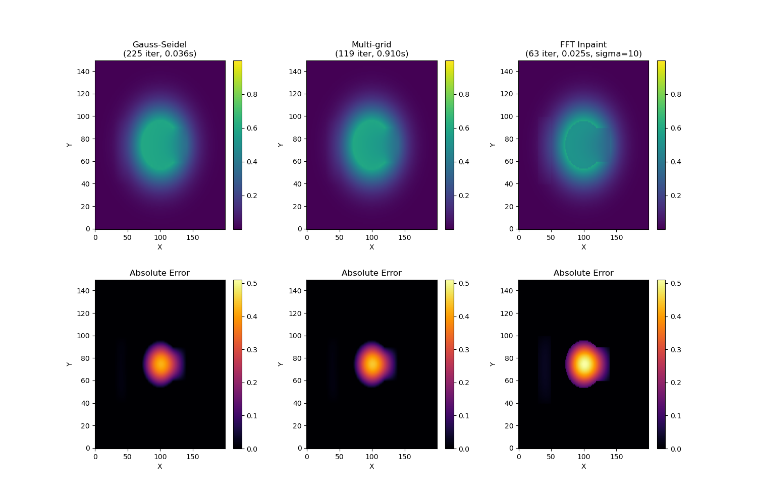
Comparing Results

Let’s visualize all results and compute errors relative to the true field:

fig, axes = matplotlib.pyplot.subplots(2, 3, figsize=(15, 10))
fig.subplots_adjust(hspace=0.3, wspace=0.3)

# Calculate errors
error_gs = numpy.abs(filled_gs - true_field)
error_mg = numpy.abs(filled_mg - true_field)
error_fft = numpy.abs(filled_fft - true_field)

vmin, vmax = true_field.min(), true_field.max()
error_max = max(error_gs.max(), error_mg.max(), error_fft.max())

# Gauss-Seidel
im0 = axes[0, 0].imshow(filled_gs.T,
                        origin='lower',
                        cmap='viridis',
                        vmin=vmin,
                        vmax=vmax,
                        aspect='auto')
axes[0, 0].set_title(f'Gauss-Seidel\n({iterations_gs} iter, {time_gs:.3f}s)')
axes[0, 0].set_xlabel('X')
axes[0, 0].set_ylabel('Y')
fig.colorbar(im0, ax=axes[0, 0])

im1 = axes[1, 0].imshow(error_gs.T,
                        origin='lower',
                        cmap='inferno',
                        vmin=0,
                        vmax=error_max,
                        aspect='auto')
axes[1, 0].set_title('Absolute Error')
axes[1, 0].set_xlabel('X')
axes[1, 0].set_ylabel('Y')
fig.colorbar(im1, ax=axes[1, 0])

# Multi-grid
im2 = axes[0, 1].imshow(filled_mg.T,
                        origin='lower',
                        cmap='viridis',
                        vmin=vmin,
                        vmax=vmax,
                        aspect='auto')
axes[0, 1].set_title(f'Multi-grid\n({iterations_mg} iter, {time_mg:.3f}s)')
axes[0, 1].set_xlabel('X')
axes[0, 1].set_ylabel('Y')
fig.colorbar(im2, ax=axes[0, 1])

im3 = axes[1, 1].imshow(error_mg.T,
                        origin='lower',
                        cmap='inferno',
                        vmin=0,
                        vmax=error_max,
                        aspect='auto')
axes[1, 1].set_title('Absolute Error')
axes[1, 1].set_xlabel('X')
axes[1, 1].set_ylabel('Y')
fig.colorbar(im3, ax=axes[1, 1])

# FFT Inpaint
im4 = axes[0, 2].imshow(filled_fft.T,
                        origin='lower',
                        cmap='viridis',
                        vmin=vmin,
                        vmax=vmax,
                        aspect='auto')
axes[0, 2].set_title(
    f'FFT Inpaint\n({iterations_fft} iter, {time_fft:.3f}s, sigma=10)')
axes[0, 2].set_xlabel('X')
axes[0, 2].set_ylabel('Y')
fig.colorbar(im4, ax=axes[0, 2])

im5 = axes[1, 2].imshow(error_fft.T,
                        origin='lower',
                        cmap='inferno',
                        vmin=0,
                        vmax=error_max,
                        aspect='auto')
axes[1, 2].set_title('Absolute Error')
axes[1, 2].set_xlabel('X')
axes[1, 2].set_ylabel('Y')
fig.colorbar(im5, ax=axes[1, 2])

fig.show()

Summary

• Gauss-Seidel: Slowest but simplest. Good for small grids or when you need fine-grained control.

• Multi-grid: Fastest for large grids. The recommended default for most use cases.

• FFT Inpaint: Excellent for creating spectrally smooth fills. Requires tuning of the sigma parameter.

• LOESS: A different approach suitable for noisy data or when local smoothing is desired.

Choose the method that best fits your grid size, performance needs, and desired fill characteristics.