2D Interpolation

This example illustrates how to perform 2D interpolation of a variable on a regular grid. The pyinterp library provides several interpolation methods, and this guide will walk you through bivariate and bicubic interpolation.

import cartopy.crs
import matplotlib
import matplotlib.pyplot
import numpy

import pyinterp
import pyinterp.backends.xarray
import pyinterp.tests

Bivariate Interpolation

Bivariate interpolation is a common method for estimating the value of a variable at a new point based on its surrounding grid points. In this section, we will perform bivariate interpolation using pyinterp.

First, we load the data and create the interpolator object. The constructor will automatically detect the longitude and latitude axes. If it fails, you can specify them by setting the units attribute to degrees_east and degrees_north. If your grid is not geodetic, set the geodetic parameter to False.

ds = pyinterp.tests.load_grid2d()
interpolator = pyinterp.backends.xarray.Grid2D(ds.mss)

Next, we define the coordinates where we want to interpolate the grid. To avoid interpolating at the grid points themselves, we shift the coordinates slightly.

mx, my = numpy.meshgrid(numpy.arange(-180, 180, 1) + 1 / 3.0,
                        numpy.arange(-89, 89, 1) + 1 / 3.0,
                        indexing='ij')

Now, we interpolate the grid to the new coordinates using the bivariate method.

mss = interpolator.bivariate(coords={
    'lon': mx.ravel(),
    'lat': my.ravel()
}).reshape(mx.shape)

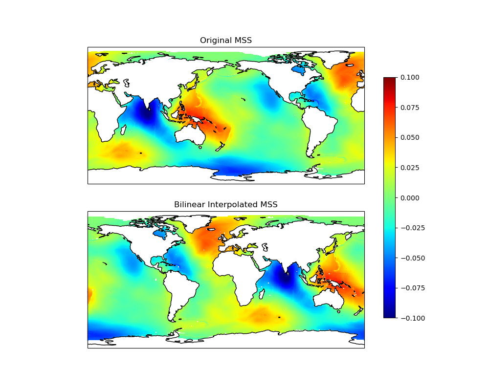
To visualize the results, we can plot the original grid and the interpolated grid.

fig = matplotlib.pyplot.figure(figsize=(10, 8))
fig.subplots_adjust(left=0.05, right=0.95, top=0.95, bottom=0.05, hspace=0.25)
ax1 = fig.add_subplot(
    211, projection=cartopy.crs.PlateCarree(central_longitude=180))
lons, lats = numpy.meshgrid(ds.lon, ds.lat, indexing='ij')
pcm = ax1.pcolormesh(lons,
                     lats,
                     ds.mss.T,
                     cmap='jet',
                     shading='auto',
                     transform=cartopy.crs.PlateCarree(),
                     vmin=-0.1,
                     vmax=0.1)
ax1.set_extent([-180, 180, -90, 90], crs=cartopy.crs.PlateCarree())
ax1.coastlines()
ax1.set_title('Original MSS')
ax2 = fig.add_subplot(212, projection=cartopy.crs.PlateCarree())
pcm = ax2.pcolormesh(mx,
                     my,
                     mss,
                     cmap='jet',
                     shading='auto',
                     transform=cartopy.crs.PlateCarree(),
                     vmin=-0.1,
                     vmax=0.1)
ax2.set_extent([-180, 180, -90, 90], crs=cartopy.crs.PlateCarree())
ax2.coastlines()
ax2.set_title('Bilinear Interpolated MSS')
fig.colorbar(pcm, ax=[ax1, ax2], shrink=0.8)

<matplotlib.colorbar.Colorbar object at 0x11e1b7290>

The bivariate method supports several interpolation techniques, including bilinear, nearest neighbor, and inverse distance weighting. Distance calculations are performed using the Haversine formula.

Bicubic Interpolation

Bicubic interpolation provides a smoother result compared to bivariate interpolation by considering a 4x4 neighborhood of grid points.

Warning

When using this interpolator, pay attention to NaN values. If the calculation window contains even a single NaN, the result of the interpolation will also be NaN, due to NaN propagation in arithmetic operations. This means the masked region effectively grows during interpolation. To avoid this behavior, you should pre-process the grid to replace or remove NaN values.

The following code performs bicubic interpolation on the same grid.

mss_bicubic = interpolator.bicubic(coords={
    'lon': mx.ravel(),
    'lat': my.ravel()
}).reshape(mx.shape)

Let’s visualize the result of the bicubic interpolation and compare it with the original data.

fig = matplotlib.pyplot.figure(figsize=(10, 8))
fig.subplots_adjust(left=0.05, right=0.95, top=0.95, bottom=0.05, hspace=0.25)
ax1 = fig.add_subplot(
    211, projection=cartopy.crs.PlateCarree(central_longitude=180))
pcm = ax1.pcolormesh(lons,
                     lats,
                     ds.mss.T,
                     cmap='jet',
                     shading='auto',
                     transform=cartopy.crs.PlateCarree(),
                     vmin=-0.1,
                     vmax=0.1)
ax1.set_extent([-180, 180, -90, 90], crs=cartopy.crs.PlateCarree())
ax1.coastlines()
ax1.set_title('Original MSS')
ax2 = fig.add_subplot(212, projection=cartopy.crs.PlateCarree())
pcm = ax2.pcolormesh(mx,
                     my,
                     mss_bicubic,
                     cmap='jet',
                     shading='auto',
                     transform=cartopy.crs.PlateCarree(),
                     vmin=-0.1,
                     vmax=0.1)
ax2.set_extent([-180, 180, -90, 90], crs=cartopy.crs.PlateCarree())
ax2.coastlines()
ax2.set_title('Bicubic Interpolated MSS')
fig.colorbar(pcm, ax=[ax1, ax2], shrink=0.8)

<matplotlib.colorbar.Colorbar object at 0x12b303c80>

The interpolation bicubic function has more parameters to define the data frame used by the spline functions and how to process the edges of the regional grids:

mss = interpolator.bicubic(
    coords={
        'lon': mx.ravel(),
        'lat': my.ravel()
    },
    nx=3,
    ny=3,
).reshape(mx.shape)

Warning

The grid provided must have strictly increasing axes to meet the specifications of the interpolation. When building the grid, specify the increasing_axes option to flip the decreasing axes and the grid automatically. For example:

interpolator = pyinterp.backends.xarray.Grid2D(
    ds.mss, increasing_axes=True)

fig = matplotlib.pyplot.figure(figsize=(10, 8))
fig.subplots_adjust(left=0.05, right=0.95, top=0.95, bottom=0.05, hspace=0.25)
ax1 = fig.add_subplot(
    211, projection=cartopy.crs.PlateCarree(central_longitude=180))
pcm = ax1.pcolormesh(lons,
                     lats,
                     ds.mss.T,
                     cmap='jet',
                     shading='auto',
                     transform=cartopy.crs.PlateCarree(),
                     vmin=-0.1,
                     vmax=0.1)
ax1.set_extent([-180, 180, -90, 90], crs=cartopy.crs.PlateCarree())
ax1.coastlines()
ax1.set_title('Original MSS')
ax2 = fig.add_subplot(212, projection=cartopy.crs.PlateCarree())
pcm = ax2.pcolormesh(mx,
                     my,
                     mss,
                     cmap='jet',
                     shading='auto',
                     transform=cartopy.crs.PlateCarree(),
                     vmin=-0.1,
                     vmax=0.1)
ax2.set_extent([-180, 180, -90, 90], crs=cartopy.crs.PlateCarree())
ax2.coastlines()
ax2.set_title('Bicubic Interpolated MSS')

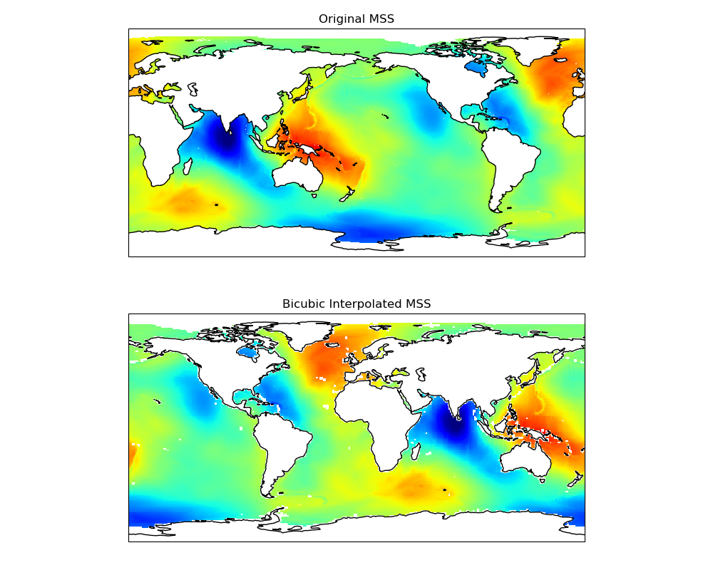
Text(0.5, 1.0, 'Bicubic Interpolated MSS')