3D Interpolation

This example demonstrates how to perform 3D interpolation on a regular grid. The pyinterp library supports both trivariate and bicubic interpolation for 3D data.

import cartopy.crs
import matplotlib
import matplotlib.pyplot
import numpy

import pyinterp
import pyinterp.backends.xarray
import pyinterp.tests

Trivariate Interpolation

Trivariate interpolation builds upon bivariate interpolation by adding a third dimension. It first performs bilinear interpolation on the 2D spatial plane (longitude and latitude), followed by linear interpolation along the time dimension. Alternatively, you can opt for nearest-neighbor interpolation on the time axis by specifying third_axis='nearest'. First, we load the 3D dataset and create the interpolator object.

ds = pyinterp.tests.load_grid3d()
interpolator = pyinterp.backends.xarray.Grid3D(ds.tcw)

Next, we define the coordinates for interpolation. To avoid interpolating at the exact grid points, we introduce a slight shift.

mx, my, mz = numpy.meshgrid(
    numpy.arange(-180, 180, 0.25) + 1 / 3.0,
    numpy.arange(-80, 80, 0.25) + 1 / 3.0,
    numpy.array(["2002-07-02T15:00:00"], dtype="datetime64"),
    indexing="ij",
)

Now, we perform the trivariate interpolation.

trivariate = interpolator.trivariate(
    {"longitude": mx.ravel(), "latitude": my.ravel(), "time": mz.ravel()}
)

Windowed Interpolators

Bicubic and spline interpolation provides smoother results compared to bilinear by using a windowed approach that considers a neighborhood of grid points within a calculation window. You can use it by passing method='bicubic' to the trivariate method or other supported methods.

interpolator = pyinterp.backends.xarray.Grid3D(ds.data_vars["tcw"])

We then perform the bicubic interpolation.

bicubic = interpolator.trivariate(
    {"longitude": mx.ravel(), "latitude": my.ravel(), "time": mz.ravel()},
    method="bicubic",
    half_window_size_x=3,
    half_window_size_y=3,
    boundary_mode="shrink",
)

To visualize the results, we reshape the output arrays and extract the longitude and latitude coordinates.

trivariate = trivariate.reshape(mx.shape).squeeze(axis=2)
bicubic = bicubic.reshape(mx.shape).squeeze(axis=2)
lons = mx[:, 0].squeeze()
lats = my[0, :].squeeze()

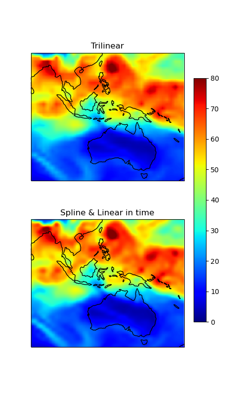
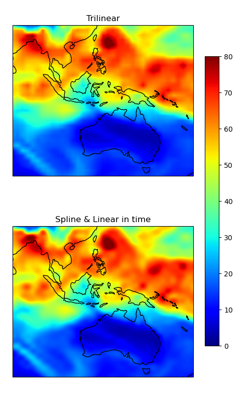
Finally, let’s plot the results of both trivariate and bicubic interpolation.

fig = matplotlib.pyplot.figure(figsize=(10, 8))
fig.subplots_adjust(left=0.05, right=0.95, top=0.95, bottom=0.05, hspace=0.25)
ax1 = fig.add_subplot(
    211, projection=cartopy.crs.PlateCarree(central_longitude=180)
)
ax1.set_extent([-180, 180, -90, 90], crs=cartopy.crs.PlateCarree())
pcm = ax1.pcolormesh(
    lons,
    lats,
    trivariate.T,
    cmap="jet",
    shading="auto",
    transform=cartopy.crs.PlateCarree(),
)
ax1.coastlines()
ax1.set_title("Trivariate Interpolation")
ax2 = fig.add_subplot(
    212, projection=cartopy.crs.PlateCarree(central_longitude=180)
)
ax2.set_extent([-180, 180, -90, 90], crs=cartopy.crs.PlateCarree())
pcm = ax2.pcolormesh(
    lons,
    lats,
    bicubic.T,
    cmap="jet",
    shading="auto",
    transform=cartopy.crs.PlateCarree(),
)
ax2.coastlines()
ax2.set_title("Bicubic Interpolation")
fig.colorbar(pcm, ax=[ax1, ax2], shrink=0.8)

<matplotlib.colorbar.Colorbar object at 0x1350ba510>

Same plot as above, but zoomed into a specific region to better highlight the differences between the two interpolation methods.

fig = matplotlib.pyplot.figure(figsize=(5, 8))
fig.subplots_adjust(left=0.05, right=0.95, top=0.95, bottom=0.05, hspace=0.25)
ax1 = fig.add_subplot(
    211, projection=cartopy.crs.PlateCarree(central_longitude=180)
)
pcm = ax1.pcolormesh(
    lons,
    lats,
    trivariate.T,
    cmap="jet",
    shading="auto",
    transform=cartopy.crs.PlateCarree(),
    vmin=0,
    vmax=80,
)
ax1.coastlines()
ax1.set_extent([80, 170, -45, 30], crs=cartopy.crs.PlateCarree())
ax1.set_title("Trilinear")

ax2 = fig.add_subplot(
    212, projection=cartopy.crs.PlateCarree(central_longitude=180)
)
pcm = ax2.pcolormesh(
    lons,
    lats,
    bicubic.T,
    cmap="jet",
    shading="auto",
    transform=cartopy.crs.PlateCarree(),
    vmin=0,
    vmax=80,
)
ax2.coastlines()
ax2.set_extent([80, 170, -45, 30], crs=cartopy.crs.PlateCarree())
ax2.set_title("Spline & Linear in time")
fig.colorbar(pcm, ax=[ax1, ax2], shrink=0.8)

<matplotlib.colorbar.Colorbar object at 0x1341a27b0>