4D Interpolation

This example demonstrates how to perform 4D interpolation on a regular grid. The pyinterp library supports both quadrivariate and bicubic interpolation for 4D data.

import cartopy.crs
import matplotlib
import matplotlib.pyplot
import numpy

import pyinterp
import pyinterp.backends.xarray
import pyinterp.tests

Quadrivariate Interpolation

Quadrivariate interpolation builds upon trivariate interpolation by adding a fourth dimension. It first performs bilinear interpolation on the 2D spatial plane (longitude and latitude), followed by linear interpolation along the third and fourth dimensions. If desired, you can use nearest-neighbor interpolation for the third and fourth dimensions by specifying third_axis=’nearest’ and fourth_axis=’nearest’. In this example, we will load a 4D dataset and create the interpolator object. First, we load the 4D dataset and create the interpolator object.

ds = pyinterp.tests.load_grid4d()
interpolator = pyinterp.backends.xarray.Grid4D(ds.pressure)

Next, we define the coordinates for interpolation.

mx, my, mz, mu = numpy.meshgrid(
    numpy.arange(-125, -70, 0.5),
    numpy.arange(25, 50, 0.5),
    numpy.datetime64("2000-01-01T12:00"),
    0.5,
    indexing="ij",
)

Now, we perform the quadrivariate interpolation.

quadrivariate = interpolator.quadrivariate(
    {
        "longitude": mx.ravel(),
        "latitude": my.ravel(),
        "time": mz.ravel(),
        "level": mu.ravel(),
    }
).reshape(mx.shape)

Windowed Interpolators

Bicubic and spline interpolation provides smoother results compared to bilinear by using a windowed approach that considers a neighborhood of grid points within a calculation window. You can use it by passing method='bicubic' to the quadrivariate method.

interpolator = pyinterp.backends.xarray.Grid4D(ds.pressure)

We then perform the bicubic interpolation.

bicubic = interpolator.quadrivariate(
    {
        "longitude": mx.ravel(),
        "latitude": my.ravel(),
        "time": mz.ravel(),
        "level": mu.ravel(),
    },
    num_threads=1,
    bounds_error=True,
    method="steffen",
    half_window_size_x=2,
    half_window_size_y=2,
    boundary_mode="shrink",
).reshape(mx.shape)

To visualize the results, we reshape the output arrays and extract the longitude and latitude coordinates.

quadrivariate = quadrivariate.squeeze(axis=(2, 3))
bicubic = bicubic.squeeze(axis=(2, 3))
lons = mx[:, 0].squeeze()
lats = my[0, :].squeeze()

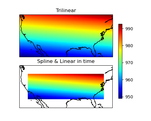
Finally, let’s plot the results of both quadrivariate and bicubic interpolation.

Note

The resolution of the example grid is low (one pixel per degree), so the bicubic interpolation may not find enough pixels at the edges, resulting in undefined values.

fig = matplotlib.pyplot.figure(figsize=(10, 8))
fig.subplots_adjust(left=0.05, right=0.95, top=0.95, bottom=0.05, hspace=0.25)
ax1 = fig.add_subplot(
    211, projection=cartopy.crs.PlateCarree(central_longitude=180)
)
ax1.set_extent(
    [lons.min(), lons.max(), lats.min(), lats.max()],
    crs=cartopy.crs.PlateCarree(),
)
pcm = ax1.pcolormesh(
    lons,
    lats,
    quadrivariate.T,
    cmap="jet",
    shading="auto",
    transform=cartopy.crs.PlateCarree(),
)
ax1.coastlines()
ax1.set_title("Quadrivariate Interpolation")
ax2 = fig.add_subplot(
    212, projection=cartopy.crs.PlateCarree(central_longitude=180)
)
ax2.set_extent(
    [lons.min(), lons.max(), lats.min(), lats.max()],
    crs=cartopy.crs.PlateCarree(),
)
pcm = ax2.pcolormesh(
    lons,
    lats,
    bicubic.T,
    cmap="jet",
    shading="auto",
    transform=cartopy.crs.PlateCarree(),
)
ax2.coastlines()
ax2.set_title("Bicubic Interpolation")
fig.colorbar(pcm, ax=[ax1, ax2], shrink=0.8)

<matplotlib.colorbar.Colorbar object at 0x1350b9be0>