Unstructured Grid Interpolation

This example illustrates the various interpolation methods available for unstructured grids, such as data from satellite tracks or other non-uniform sources.

The core of unstructured grid interpolation in pyinterp is the pyinterp.RTree class, which uses an R-tree data structure for efficient spatial queries.

First, we’ll create a synthetic dataset to represent our unstructured grid.

import cartopy.crs
import cartopy.feature
import matplotlib.pyplot
import numpy

import pyinterp

The R-tree can be configured to work with different geodetic systems. The default is WGS-84. Here, we’ll use the default.

mesh = pyinterp.RTree()

We will create a synthetic field of data to simulate measurements from an unstructured grid.

def field(lon, lat):
    """A synthetic field of data."""
    return (
        numpy.sin(numpy.radians(lon) * 3) * numpy.cos(numpy.radians(lat) * 2) +
        0.5 * numpy.sin(numpy.radians(lon) * 5) *
        numpy.sin(numpy.radians(lat) * 4))

Now, we generate random longitude and latitude points and populate our R-tree with these points and their corresponding data values. The packing() method is the most efficient way to build the tree from a complete dataset at once.

N_POINTS = 2000
X0, X1 = 80, 170
Y0, Y1 = -45, 30
generator = numpy.random.Generator(numpy.random.PCG64(0))
lons = generator.uniform(low=X0, high=X1, size=(N_POINTS, ))
lats = generator.uniform(low=Y0, high=Y1, size=(N_POINTS, ))
data = field(lons, lats)

mesh.packing(numpy.vstack((lons, lats)).T, data)

For our interpolation, we need a grid where we want to estimate the values. We’ll create a regular grid for this purpose.

STEP = 0.5
mx, my = numpy.meshgrid(numpy.arange(X0, X1 + STEP, STEP),
                        numpy.arange(Y0, Y1 + STEP, STEP),
                        indexing='ij')

Interpolation Methods

pyinterp offers several methods for interpolating data from an unstructured grid. We will now apply and visualize each of them.

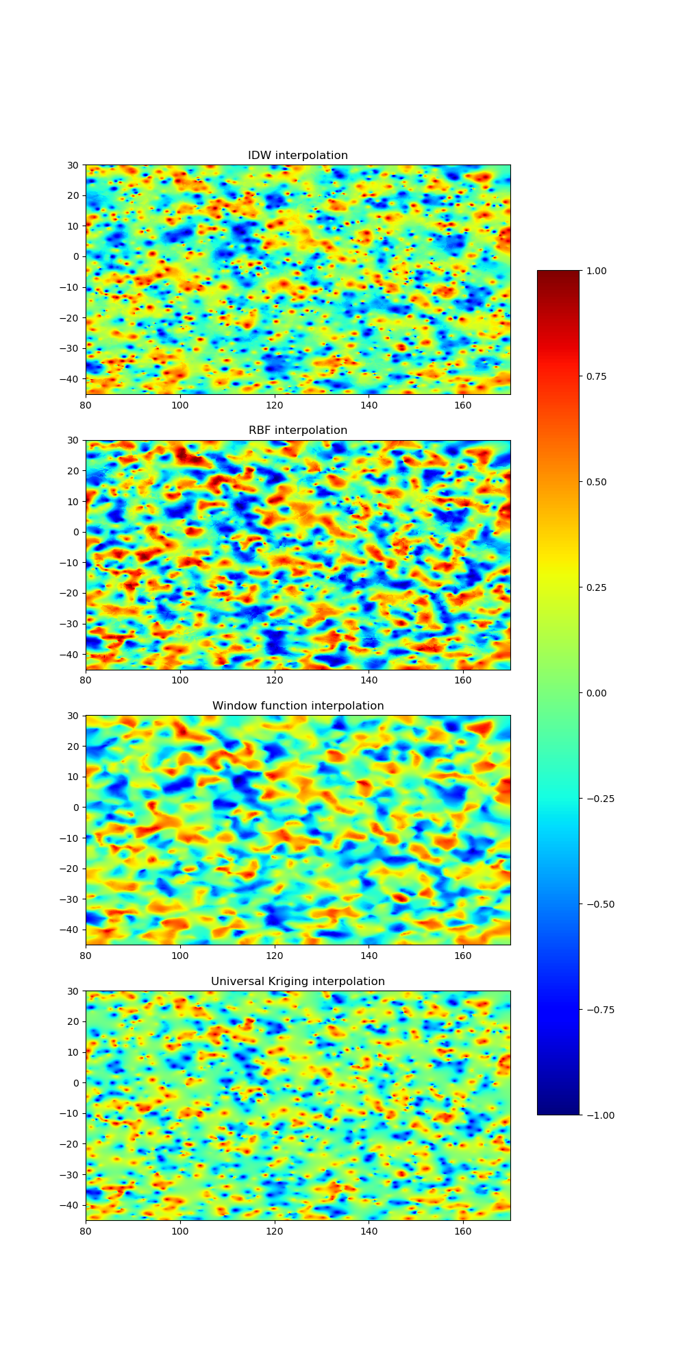
Inverse Distance Weighting (IDW), Radial Basis Function (RBF), and Kriging are all interpolation methods used to estimate a value for a target location based on the values of surrounding sample points. However, each method approaches this estimation differently.

IDW uses a weighted average of the surrounding sample points, where the weight assigned to each point is inversely proportional to its distance from the target location. The further away a sample point is from the target location, the less influence it has on the estimated value. This method is relatively simple to implement and computationally efficient, but it can produce over-smoothed results in areas with a lot of sample points and under-smoothed results in areas with few sample points.

The Window Function method, much like IDW, uses a weighted average of the surrounding sample points. However, instead of the weight being solely determined by the inverse distance, it is determined by a kernel function (the “window”). This function gives the most weight to points at the center of the window and progressively less weight to points further away. This can sometimes provide a smoother result than IDW.

RBF, on the other hand, models the spatial relationship between sample points and the target location by using a mathematical function (radial basis function) that is based on the distance between the points. The radial basis function is usually Gaussian, multiquadric, or inverse multiquadric. The estimated value at the target location is obtained by summing up the weighted contributions of all sample points. This method is more flexible than IDW as it can produce both smooth and non-smooth surfaces depending on the chosen radial basis function. However, it can be computationally expensive and may produce artifacts in areas with sparse or clustered sample points.

Kriging is a geostatistical interpolation method that uses a variogram to model the spatial correlation between sample points. The variogram describes how the similarity between sample points decreases as the distance between them increases. The estimated value at the target location is obtained by a weighted average of the surrounding sample points, where the weights are determined by the variogram model. This method is considered to be the most accurate interpolation method as it provides an optimal and unbiased estimate of the value at the target location. However, it is also the most computationally expensive and requires a good understanding of the underlying spatial structure of the data.

In summary, the choice of interpolation method is a trade-off between simplicity, computational cost, and the quality of the results.

• IDW is a good starting point as it is simple and fast.

• The Window Function can provide a smoother alternative to IDW.

• RBF offers more flexibility but at a higher computational cost and with a risk of artifacts.

• Kriging is the most accurate method but also the most complex and computationally intensive, requiring a good understanding of the data’s spatial structure.

In this notebook, we will compare the results of these four interpolation methods on a synthetic dataset.

Inverse Distance Weighting (IDW)

idw, _ = mesh.inverse_distance_weighting(
    numpy.vstack((mx.ravel(), my.ravel())).T,
    within=False,
    k=11,
    radius=None,
    num_threads=0,
)
idw = idw.reshape(mx.shape)

Radial Basis Function (RBF)

rbf, _ = mesh.radial_basis_function(numpy.vstack((mx.ravel(), my.ravel())).T,
                                    within=False,
                                    k=11,
                                    rbf='multiquadric',
                                    epsilon=None,
                                    smooth=0,
                                    num_threads=0)
rbf = rbf.reshape(mx.shape)

Window Function

wf, _ = mesh.window_function(numpy.vstack((mx.ravel(), my.ravel())).T,
                             within=False,
                             k=11,
                             wf='parzen',
                             radius=None,
                             num_threads=0)
wf = wf.reshape(mx.shape)

Kriging

kriging, _ = mesh.kriging(numpy.vstack((mx.ravel(), my.ravel())).T,
                          within=False,
                          k=11,
                          radius=None,
                          covariance='gaussian',
                          drift_function='linear',
                          num_threads=0)
kriging = kriging.reshape(mx.shape)

Visualization of Results

Finally, let’s visualize the original scattered data and the results of the different interpolation methods on a map.

fig = matplotlib.pyplot.figure(figsize=(20, 10))
fig.patch.set_alpha(0.0)
gs = fig.add_gridspec(2, 4)
ax1 = fig.add_subplot(gs[0, 0], projection=cartopy.crs.PlateCarree())
ax2 = fig.add_subplot(gs[0, 1], projection=cartopy.crs.PlateCarree())
ax3 = fig.add_subplot(gs[0, 2], projection=cartopy.crs.PlateCarree())
ax4 = fig.add_subplot(gs[0, 3], projection=cartopy.crs.PlateCarree())
ax5 = fig.add_subplot(gs[1, 0], projection=cartopy.crs.PlateCarree())
ax6 = fig.add_subplot(gs[1, 1], projection=cartopy.crs.PlateCarree())
ax7 = fig.add_subplot(gs[1, 2], projection=cartopy.crs.PlateCarree())
ax8 = fig.add_subplot(gs[1, 3], projection=cartopy.crs.PlateCarree())


# Common plotting function
def plot_grid(ax, grid, title, cmap, vmin, vmax):
    """Helper function to plot interpolated grids."""
    pcm = ax.pcolormesh(mx,
                        my,
                        grid,
                        cmap=cmap,
                        transform=cartopy.crs.PlateCarree(),
                        vmin=vmin,
                        vmax=vmax)
    ax.coastlines()
    ax.add_feature(cartopy.feature.BORDERS, linestyle='-')
    ax.set_title(title)
    return pcm


# Plotting each interpolation result
true = field(mx, my)
plot_grid(ax1, idw, 'Inverse Distance Weighting', 'viridis', -1, 1)
plot_grid(ax2, rbf, 'Radial Basis Function', 'viridis', -1, 1)
plot_grid(ax3, wf, 'Window Function', 'viridis', -1, 1)
plot_grid(ax4, kriging, 'Kriging', 'viridis', -1, 1)

# Plotting errors
error_idw = numpy.where(true != 0, (idw - true) / true, 0)
error_rbf = numpy.where(true != 0, (rbf - true) / true, 0)
error_wf = numpy.where(true != 0, (wf - true) / true, 0)
error_kriging = numpy.where(true != 0, (kriging - true) / true, 0)

plot_grid(ax5, error_idw, 'IDW Relative Error', 'RdBu_r', -0.5, 0.5)
plot_grid(ax6, error_rbf, 'RBF Relative Error', 'RdBu_r', -0.5, 0.5)
plot_grid(ax7, error_wf, 'Window Function Relative Error', 'RdBu_r', -0.5, 0.5)
plot_grid(ax8, error_kriging, 'Kriging Relative Error', 'RdBu_r', -0.5, 0.5)

fig.tight_layout()
matplotlib.pyplot.show()