Geohash

Geohashing is a geocoding method used to encode geographic coordinates (latitude and longitude) into a short string of digits and letters. This string, also known as a geohash, delineates a rectangular area on a map, called a cell. The longer the string, the smaller the cell and the more precise the location.

This library provides two ways to work with geohashes:

• The pyinterp.GeoHash class allows for an object-oriented manipulation of a geohash.

• The pyinterp.geohash module provides functions for vectorized computation of geohashes.

In general, you should use the pyinterp.GeoHash class when you want to manipulate a few geohashes, and the pyinterp.geohash module when you want to process a large number of geohashes stored in numpy arrays.

The following sections will demonstrate how to use both approaches.

Geohash Grid

First, let’s define a few functions to visualize geohash grids. These functions are for illustrative purposes and are not part of the pyinterp library.

import timeit

import cartopy.crs
import matplotlib.colors
import matplotlib.patches
import matplotlib.pyplot
import numpy
import pandas

import pyinterp

Writing a visualization routine for GeoHash grids.

def _sort_colors(colors):
    """Sort colors by hue, saturation, value and name in descending order."""
    by_hsv = sorted(
        (tuple(matplotlib.colors.rgb_to_hsv(matplotlib.colors.to_rgb(color))),
         name) for name, color in colors.items())
    return [name for hsv, name in reversed(by_hsv)]


def _plot_box(ax, code, color, caption=True):
    """Plot a GeoHash bounding box."""
    box = pyinterp.GeoHash.from_string(code.decode()).bounding_box()
    x0 = box.min_corner.lon
    x1 = box.max_corner.lon
    y0 = box.min_corner.lat
    y1 = box.max_corner.lat
    dx = x1 - x0
    dy = y1 - y0
    box = matplotlib.patches.Rectangle((x0, y0),
                                       dx,
                                       dy,
                                       alpha=0.5,
                                       color=color,
                                       ec='black',
                                       lw=1,
                                       transform=cartopy.crs.PlateCarree())
    ax.add_artist(box)
    if not caption:
        return
    rx, ry = box.get_xy()
    cx = rx + box.get_width() * 0.5
    cy = ry + box.get_height() * 0.5
    ax.annotate(code.decode(), (cx, cy),
                color='w',
                weight='bold',
                fontsize=16,
                ha='center',
                va='center')


def plot_geohash_grid(precision,
                      polygon=None,
                      caption=True,
                      color_list=None,
                      inc=7):
    """Plot geohash bounding boxes."""
    color_list = color_list or matplotlib.colors.CSS4_COLORS
    fig = matplotlib.pyplot.figure(figsize=(24, 12))
    ax = fig.add_subplot(1, 1, 1, projection=cartopy.crs.PlateCarree())
    if polygon is not None:
        box = polygon.envelope() if isinstance(
            polygon, pyinterp.geodetic.Polygon) else polygon

        ax.set_extent(
            [
                box.min_corner.lon,
                box.max_corner.lon,
                box.min_corner.lat,
                box.max_corner.lat,
            ],
            crs=cartopy.crs.PlateCarree(),
        )
    else:
        box = None
    colors = _sort_colors(color_list)
    ic = 0
    codes = pyinterp.geohash.bounding_boxes(polygon, precision=precision)

    color_codes = {codes[0][0]: colors[ic]}
    for item in codes:
        prefix = item[precision - 1]
        if prefix not in color_codes:
            ic += inc
            color_codes[prefix] = colors[ic % len(colors)]
        _plot_box(ax, item, color_codes[prefix], caption)
    ax.stock_img()
    ax.coastlines()
    ax.grid()

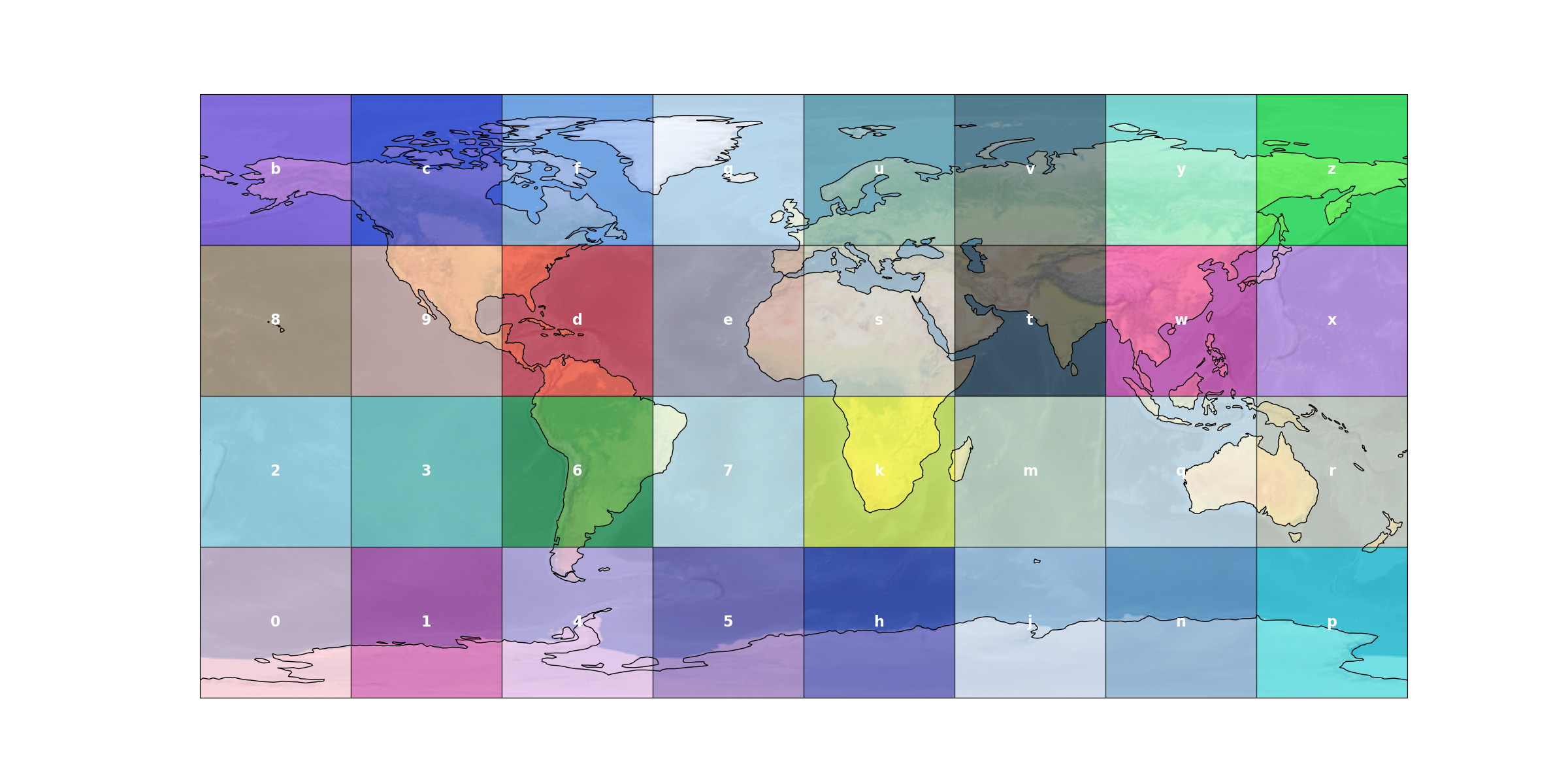
Bounds of geohash with a precision of 1 character.

plot_geohash_grid(1)

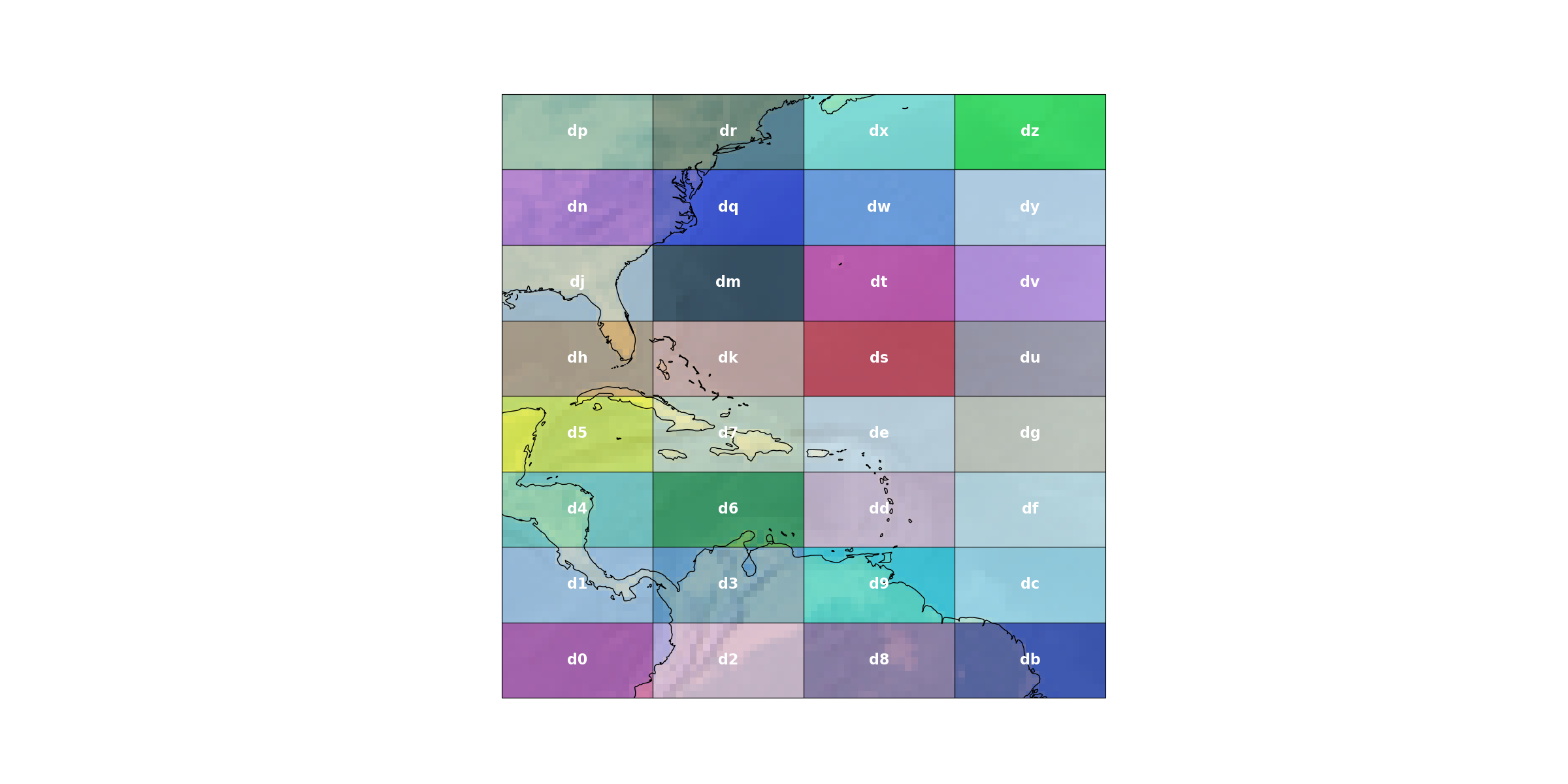
Bounds of the geohash d with a precision of two characters.

plot_geohash_grid(2, polygon=pyinterp.GeoHash.from_string('d').bounding_box())

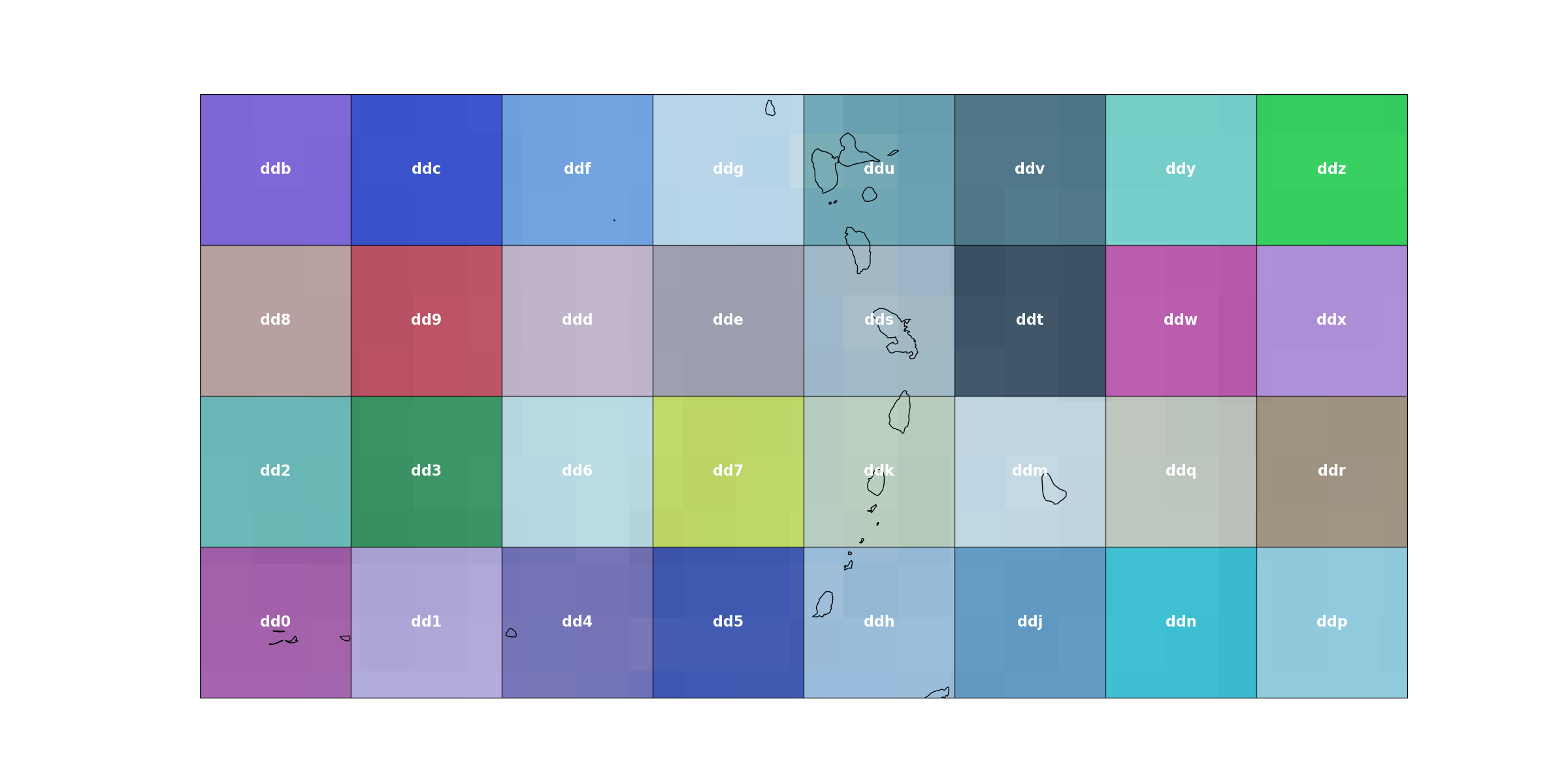
Bounds of the geohash dd with a precision of three characters.

plot_geohash_grid(3, polygon=pyinterp.GeoHash.from_string('dd').bounding_box())

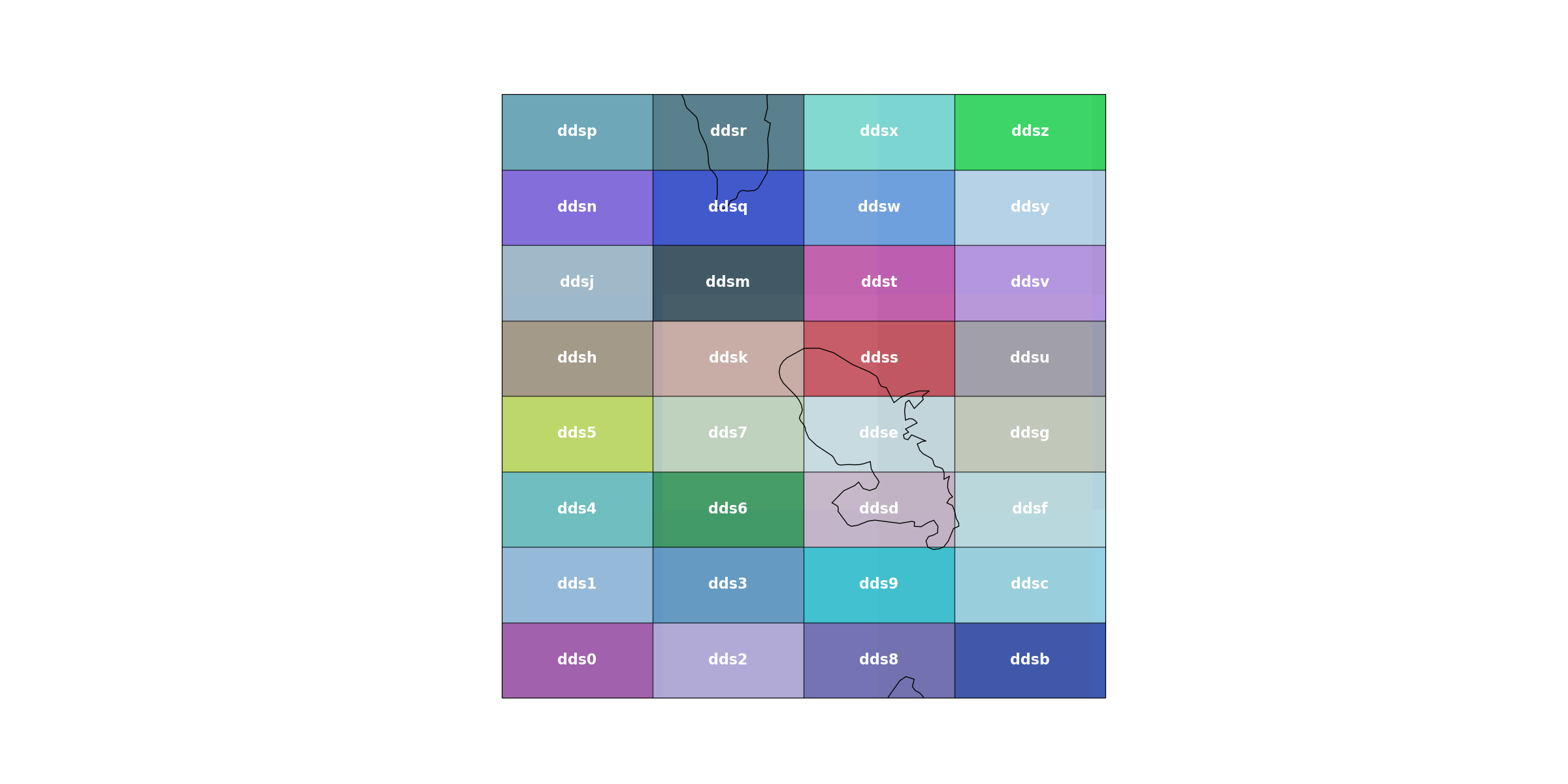
Bounds of the geohash dds with a precision of four characters.

plot_geohash_grid(4,
                  polygon=pyinterp.GeoHash.from_string('dds').bounding_box())

Object-Oriented Interface

The pyinterp.GeoHash class allows for an object-oriented manipulation of a geohash. You can create a geohash from a longitude and latitude, and then access its properties.

code = pyinterp.GeoHash(-67.5, 22.5, precision=4)
print(f'The geohash is {code!s}')
print(f'The precision of the geohash is {code.precision()}')
print(f'The number of bits is {code.number_of_bits()}')
print(f'The center of the cell is at {code.center()}')

The geohash is ds00
The precision of the geohash is 4
The number of bits is 20
The center of the cell is at (-67.3242, 22.5879)

You can also use this class to get the neighboring geohash codes.

[str(item) for item in code.neighbors()]

['ds01', 'ds03', 'ds02', 'debr', 'debp', 'd7zz', 'dkpb', 'dkpc']

Vectorized Interface

On the other hand, when you want to encode a large volume of data, you should use functions that work on numpy arrays.

Generation of dummy data

SIZE = 1_000_000
generator = numpy.random.Generator(numpy.random.PCG64(0))
lon = generator.uniform(-180, 180, SIZE)
lat = generator.uniform(-80, 80, SIZE)
measures = generator.random(SIZE)

Encoding the data is done using the pyinterp.geohash.encode() function.

codes = pyinterp.geohash.encode(lon, lat, precision=4)
print(codes)

[b'mng5' b'fhv0' b'87d7' ... b'9hfj' b'3yvj' b'5ghs']

As you can see, the resulting codes are encoding as numpy byte arrays. This is to save memory and speed up the processing. This algorithm is very fast, which makes it possible to process a lot of data quickly.

The following benchmark measures the time it takes to encode the coordinates into geohashes.

elapsed = timeit.timeit('pyinterp.geohash.encode(lon, lat, precision=12)',
                        number=50,
                        globals={
                            'pyinterp': pyinterp,
                            'lon': lon,
                            'lat': lat
                        }) / 50
print(f'Elapsed time: {elapsed:.6f} seconds')

Elapsed time: 0.036425 seconds

The inverse operation is also possible using the pyinterp.geohash.decode() function.

lon, lat = pyinterp.geohash.decode(codes)

You can also use the pyinterp.geohash.transform() to transform geohashes from one precision to another.

codes = pyinterp.geohash.transform(codes, precision=1)
print(codes)

[b'0' b'1' b'2' b'3' b'4' b'5' b'6' b'7' b'8' b'9' b'b' b'c' b'd' b'e'
 b'f' b'g' b'h' b'j' b'k' b'm' b'n' b'p' b'q' b'r' b's' b't' b'u' b'v'
 b'w' b'x' b'y' b'z']

codes = pyinterp.geohash.transform(codes, precision=3)
print(codes)

[b'000' b'001' b'004' ... b'zzv' b'zzy' b'zzz']

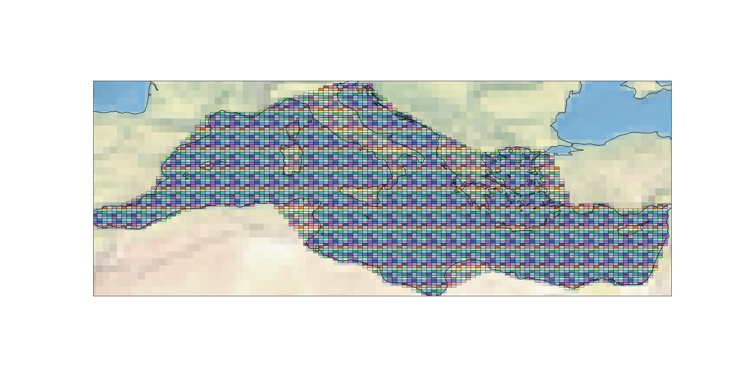
The pyinterp.geohash.bounding_boxes() function allows calculating the geohash codes contained in a box or a polygon. This function allows, for example, to obtain all the geohash codes present on the Mediterranean Sea.

MEDITERRANEAN_SEA = [(-1.43504, 35.38124), (-1.68901, 35.18381),
                     (-1.93947, 35.18664), (-2.18994, 35.18945),
                     (-2.44041, 35.19223), (-2.69089, 35.19498),
                     (-3.19185, 35.20043), (-3.44234, 35.20312),
                     (-4.19382, 35.21103), (-4.44432, 35.21363),
                     (-4.69483, 35.21619), (-4.94221, 35.42047),
                     (-5.18954, 35.62438), (-5.18619, 35.82515),
                     (-5.18272, 36.02538), (-5.17911, 36.22509),
                     (-4.92467, 36.42114), (-4.41929, 36.61311),
                     (-4.16856, 36.60978), (-3.91785, 36.60641),
                     (-3.66714, 36.60302), (-3.41643, 36.59959),
                     (-1.64252, 37.35734), (-0.61682, 38.11193),
                     (-0.05974, 39.61617), (-0.05188, 39.80296),
                     (0.47608, 40.34624), (1.0068, 40.88237),
                     (1.26823, 41.05687), (3.17405, 43.12814),
                     (3.95946, 43.44167), (4.21176, 43.4303),
                     (4.46402, 43.41885), (5.4578, 43.20103),
                     (7.00043, 43.46998), (7.2684, 43.62615),
                     (8.32692, 44.07445), (8.59664, 44.22593),
                     (8.86679, 44.37629), (9.11878, 44.36187),
                     (12.30323, 45.45208), (12.82897, 45.57254),
                     (13.35502, 45.69103), (13.60653, 45.6726),
                     (14.56628, 45.29165), (14.77339, 44.96545),
                     (16.35039, 43.4468), (16.83351, 43.25904),
                     (17.31681, 43.07169), (18.26742, 42.54036),
                     (18.50146, 42.36803), (18.73581, 42.19562),
                     (19.45557, 41.83742), (22.59567, 40.39801),
                     (23.86967, 40.66103), (24.38198, 40.79528),
                     (25.14395, 40.91539), (25.39346, 40.90312),
                     (25.87922, 40.72341), (27.3756, 40.65146),
                     (27.3629, 40.4972), (27.35049, 40.34214),
                     (28.89327, 36.67855), (30.6478, 36.80647),
                     (30.89745, 36.80017), (31.14709, 36.79388),
                     (31.63983, 36.61137), (32.1328, 36.42873),
                     (34.38535, 36.54538), (34.64117, 36.70704),
                     (34.89068, 36.70094), (35.89499, 36.84229),
                     (36.14443, 36.83607), (36.13812, 36.67067),
                     (35.84461, 35.31519), (35.83989, 35.14037),
                     (35.83535, 34.96453), (35.83096, 34.78764),
                     (35.82673, 34.60973), (35.82266, 34.43077),
                     (35.56521, 34.07323), (35.30493, 33.52656),
                     (35.04582, 32.96983), (34.78535, 32.21131),
                     (34.53086, 31.82665), (34.27678, 31.43758),
                     (34.02492, 31.24227), (33.77499, 31.24401),
                     (33.52506, 31.24576), (33.27513, 31.24751),
                     (33.02519, 31.24927), (32.77526, 31.25102),
                     (32.52532, 31.25279), (32.27538, 31.25455),
                     (30.52777, 31.46553), (29.27227, 30.87518),
                     (29.0223, 30.87679), (28.27422, 31.08288),
                     (27.52624, 31.28865), (26.5284, 31.49606),
                     (25.53067, 31.70343), (25.28069, 31.70546),
                     (24.03548, 32.11364), (23.28805, 32.31846),
                     (20.02259, 30.93524), (19.77083, 30.7316),
                     (19.51917, 30.52699), (19.26761, 30.32143),
                     (19.01759, 30.32277), (18.51909, 30.5327),
                     (17.77237, 30.94967), (17.0241, 31.15993),
                     (16.02586, 31.37173), (15.77581, 31.37348),
                     (15.52992, 31.78362), (13.79181, 32.80886),
                     (12.7914, 32.81862), (12.54129, 32.82104),
                     (12.04387, 33.02684), (11.54655, 33.23236),
                     (10.30532, 33.84446), (10.05858, 34.04584),
                     (10.06218, 34.24361), (7.87667, 36.9875),
                     (7.12516, 37.00275), (6.87464, 37.00779),
                     (5.86671, 36.83664), (5.61618, 36.84139),
                     (5.36563, 36.84612), (5.11508, 36.85081),
                     (4.86453, 36.85549), (3.61163, 36.87846),
                     (2.60396, 36.70273), (2.35336, 36.70699),
                     (1.34599, 36.52884), (0.07965, 35.95831),
                     (-0.67601, 35.77038), (-1.43504, 35.38124)]
polygon = pyinterp.geodetic.Polygon(
    [pyinterp.geodetic.Point(lon, lat) for lon, lat in MEDITERRANEAN_SEA])

precision = 4
plot_geohash_grid(precision, polygon=polygon, caption=False)

Density calculation

Finally, we will calculate the density of points in each geohash cell. For this, we will use the pyinterp.geohash.encode() function to get the geohash of each point, and then we will group the points by geohash and count the number of points in each cell.

df = pandas.DataFrame({
    'lon': lon,
    'lat': lat,
    'measures': measures,
    'geohash': pyinterp.geohash.encode(lon, lat, precision=3)
})
df.set_index('geohash', inplace=True)
df = df.groupby('geohash').count()['measures'].rename('count').to_frame()

Then, we calculate the density of points in each cell by dividing the number of points by the area of the cell in square kilometers.

df['density'] = df['count'] / (
    pyinterp.geohash.area(df.index.values.astype('S')) / 1e6)

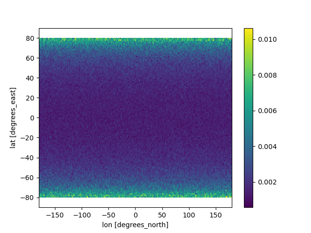
Finally, we can visualize the density of points on a map. For this, we will use the pyinterp.geohash.to_xarray() function to convert the geohash and the density into an xarray.DataArray.

array = pyinterp.geohash.to_xarray(df.index.values.astype('S'),
                                   df.density.values)
array = array.where(array != 0, numpy.nan)

fig = matplotlib.pyplot.figure(figsize=(10, 5))
ax = fig.add_subplot(111, projection=cartopy.crs.PlateCarree())
array.plot(ax=ax,
           transform=cartopy.crs.PlateCarree(),
           cmap='viridis',
           robust=True)
ax.coastlines()
ax.gridlines(draw_labels=True)
ax.set_global()