

Note
Go to the end to download the full example code or to run this example in your browser via Binder.
Orbit Interpolation#
This example demonstrates how to use pyinterp to interpolate satellite
orbits. The library can propagate orbit ephemerides from a template file that
contains satellite positions for a single orbit cycle. This is useful for
simulations and other applications that require accurate orbit propagation over
time.
To begin, we will load the orbit ephemeris from a test file.
import pathlib

import cartopy.crs as ccrs
import matplotlib.pyplot as plt
import numpy as np
import pandas as pd

import pyinterp.orbit
import pyinterp.tests


def load_test_ephemeris(
    filename: pathlib.Path,
) -> tuple[float, np.ndarray, np.ndarray, np.ndarray, np.timedelta64]:
    """Loads the ephemeris from a text file.

    Args:
        filename: Name of the file to be loaded.

    Returns:
        A tuple containing the height of the orbit, the ephemeris, and the
        duration of the cycle.

    """
    with open(filename, encoding="utf-8") as stream:
        lines = stream.readlines()

    def to_dict(comments) -> dict[str, float]:
        """Returns a dictionary describing the parameters of the orbit."""
        result = {}
        for item in comments:
            if not item.startswith("#"):
                raise ValueError("Comments must start with #")
            key, value = item[1:].split("=")
            result[key.strip()] = float(value)
        return result

    # The first two lines are the header and contain the height and the
    # duration of the cycle in fractional days.
    settings = to_dict(lines[:2])
    del lines[:2]

    # The rest of the lines are the ephemeris.
    ephemeris = np.loadtxt(
        lines,
        delimiter=" ",
        dtype={
            "names": ("time", "longitude", "latitude", "height"),
            "formats": ("f8", "f8", "f8", "f8"),
        },
    )

    return (
        settings["height"],
        ephemeris["longitude"],
        ephemeris["latitude"],
        ephemeris["time"].astype("timedelta64[s]"),
        np.timedelta64(int(settings["cycle_duration"] * 86400.0 * 1e9), "ns"),
    )
Loading the Ephemeris#
First, we set the path to the test file and load the ephemeris data.
ephemeris_path = pyinterp.tests.ephemeris_path()
ephemeris = load_test_ephemeris(ephemeris_path)
Calculating Orbit Properties#
With the ephemeris loaded, we can compute the orbit properties using the
pyinterp.calculate_orbit() function.
orbit = pyinterp.orbit.calculate_orbit(*ephemeris)
The resulting pyinterp.Orbit object provides methods to access
various orbit properties. For example, you can get the number of passes per
cycle:
print(f"Passes per cycle: {orbit.passes_per_cycle()}")
Passes per cycle: 28
You can also get the cycle duration and the orbit duration:
print(f"Cycle duration: {orbit.cycle_duration().astype('m8[ms]').item()}")
print(f"Orbit duration: {orbit.orbit_duration().astype('m8[ms]').item()}")
Cycle duration: 23:25:23.172000
Orbit duration: 1:40:23.083000
The duration of a specific pass can also be retrieved:
print(f"Pass 2 duration: {orbit.pass_duration(2).astype('m8[ms]').item()}")
Pass 2 duration: 0:55:44.351000
Encoding and Decoding Pass Numbers#
A utility function is provided to compute an absolute pass number from a relative pass number and a cycle number. This is useful for storing pass information in a database or for indexing passes in a file.
absolute_pass_number = orbit.encode_absolute_pass_number(
    cycle_number=11, pass_number=2
)
print(f"Absolute pass number: {absolute_pass_number}")
Absolute pass number: 282
You can decode the absolute pass number to get the cycle and pass numbers:
cycle_number, pass_number = orbit.decode_absolute_pass_number(
    absolute_pass_number
)
print(f"Cycle: {cycle_number}, Pass: {pass_number}")
Cycle: 11, Pass: 2
Interpolating the Orbit#
The next step is to interpolate the orbit ephemerides over time to get the satellite positions for a given relative pass number.
Note
You can iterate over the relative pass numbers for a given time period
using the pyinterp.Orbit.iterate() method.
for cycle_number, pass_number, first_location_date in orbit.iterate(
        start_date, end_date):
    ...
pass_ = pyinterp.orbit.calculate_pass(2, orbit)
assert pass_ is not None
pd.DataFrame(
    {
        "time": pass_.time,
        "lon_nadir": pass_.lon_nadir,
        "lat_nadir": pass_.lat_nadir,
    }
)
The pyinterp.Pass object contains the satellite’s nadir positions
for the given pass, including:
Nadir longitude (in degrees)
Nadir latitude (in degrees)
Time for each position (as a
numpy.datetime64array)Along-track distance (in meters)
It also provides the coordinates of the satellite at the equator:
print(f"Equator coordinates: {pass_.equator_coordinates}")
Equator coordinates: EquatorCoordinates(longitude=59.20360095529903, time=np.timedelta64(3087382,'ms'))
Note
The pass_ variable will be None if the pass number is outside the
bounding box defined during the instantiation of the
pyinterp.Orbit object.
Calculating the Swath#
Finally, we can calculate the satellite positions over a swath for a given pass.
swath = pyinterp.orbit.calculate_swath(pass_)
The pyinterp.Swath object contains the properties of the pass,
similar to the pyinterp.Pass object. Additionally, it includes
the coordinates of the satellite over the swath for each location on the
nadir track.
pd.DataFrame(
    {
        "time": swath.time,
        "lon_nadir": swath.lon_nadir,
        "lat_nadir": swath.lat_nadir,
    }
)
The following DataFrame shows the longitude and latitude coordinates of the
satellite for the first two lines of the swath. The index x_ac represents
the across-track distance in meters.
df = pd.DataFrame(
    {
        "lon_0": swath.lon[0, :],
        "lon_1": swath.lon[1, :],
        "lat_0": swath.lat[0, :],
        "lat_1": swath.lat[1, :],
    },
    index=swath.x_ac[0, :],
)
df.index.name = "x_ac"
df
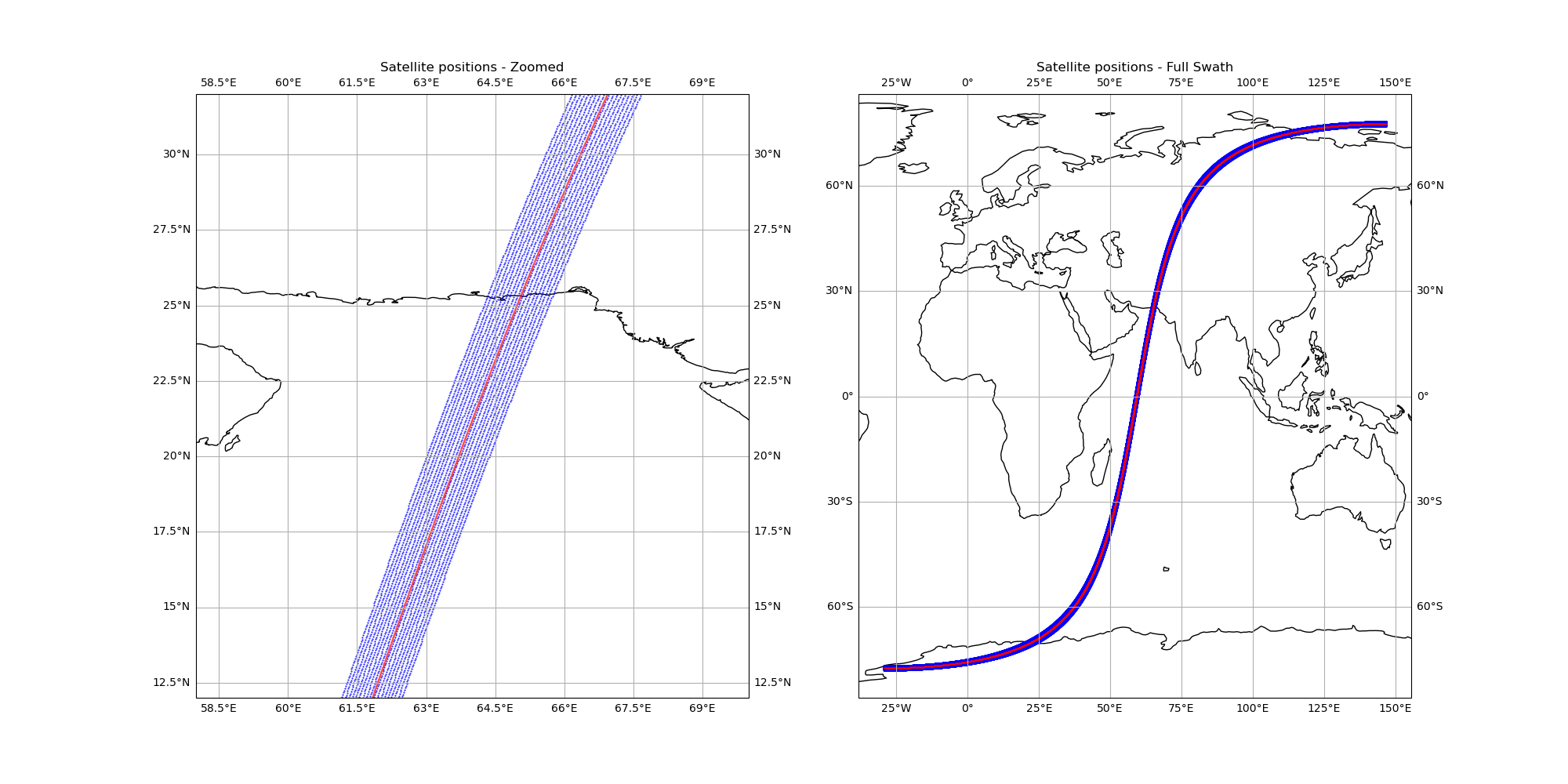
Visualizing the Swath#
We can now plot the satellite positions over the swath.
fig, (ax1, ax2) = plt.subplots(
    1, 2, figsize=(20, 10), subplot_kw={"projection": ccrs.PlateCarree()}
)
fig.subplots_adjust(left=0.05, right=0.95, top=0.95, bottom=0.05, wspace=0.1)

# Zoomed plot
ax1.set_extent([58, 70, 12, 32], crs=ccrs.PlateCarree())
ax1.plot(
    swath.lon[::4, ::4].ravel(),
    swath.lat[::4, ::4].ravel(),
    "b.",
    markersize=1,
)
ax1.plot(swath.lon_nadir, swath.lat_nadir, "r.", markersize=0.5)
ax1.set_title("Satellite positions - Zoomed")
ax1.coastlines()
ax1.gridlines(draw_labels=True)

# Full swath plot
ax2.plot(swath.lon.ravel(), swath.lat.ravel(), "b.", markersize=1)
ax2.plot(swath.lon_nadir, swath.lat_nadir, "r.", markersize=0.5)
ax2.set_title("Satellite positions - Full Swath")
ax2.coastlines()
ax2.gridlines(draw_labels=True)
ax1.set_aspect("auto")
ax2.set_aspect("auto")
Total running time of the script: (0 minutes 1.141 seconds)