Robust Statistics with Histograms and T-Digest

The mean of a bin is sensitive to outliers and hides the shape of skewed distributions. pyinterp.Histogram2D keeps, in each bin, a compact summary of the whole distribution built with the T-Digest algorithm, and pyinterp.TDigest does the same for a 1D stream of values. In this example, you will learn how to map per-bin medians and quantiles, how to merge digests computed on separate batches, and how the compression parameter trades accuracy for memory.

import pickle

import matplotlib.pyplot
import numpy

import pyinterp
import pyinterp.tests

rng = numpy.random.default_rng(0)

Contaminated Drifter Speeds

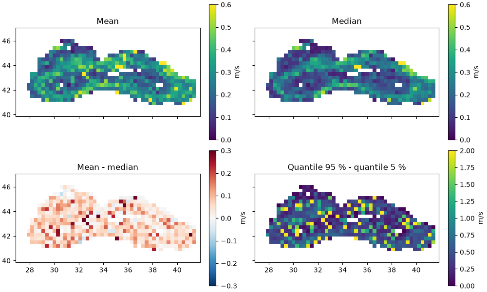
We reuse the drifter velocities of the Black Sea, already binned in the Binning example, and compute their speed. To mimic spurious positioning fixes, 3 % of the speeds are replaced by values between 1 and 3 m/s, well above the typical speed of the currents.

ds = pyinterp.tests.load_aoml()
lon = ds.lon.values
lat = ds.lat.values
speed = numpy.hypot(ds.ud.values, ds.vd.values)

outliers = rng.random(speed.size) < 0.03
noisy = speed.copy()
noisy[outliers] = rng.uniform(1.0, 3.0, outliers.sum())

Per-Bin Distributions

A pyinterp.Histogram2D is defined by two axes, like pyinterp.Binning2D. Each value pushed is assigned to the bin of the nearest grid node, and NaN values are ignored. Besides the mean, the quantile method estimates any quantile of the values in each bin. Empty bins are set to NaN.

x_axis = pyinterp.Axis(numpy.arange(27, 42, 0.3), period=360.0)
y_axis = pyinterp.Axis(numpy.arange(40, 47, 0.3))

hist = pyinterp.Histogram2D(x_axis, y_axis)
hist.push(lon, lat, noisy)

mean = hist.mean()
median = hist.quantile(0.5)
q05 = hist.quantile(0.05)
q95 = hist.quantile(0.95)

The same histogram built from the clean speeds gives the reference against which we measure the bias introduced by the outliers.

reference = pyinterp.Histogram2D(x_axis, y_axis)
reference.push(lon, lat, speed)
ref_median = reference.quantile(0.5)

print(f'Mean absolute bias of the mean:   '
      f'{numpy.nanmean(numpy.abs(mean - ref_median)):.3f} m/s')
print(f'Mean absolute bias of the median: '
      f'{numpy.nanmean(numpy.abs(median - ref_median)):.3f} m/s')

Mean absolute bias of the mean:   0.077 m/s
Mean absolute bias of the median: 0.008 m/s

The mean is pulled up wherever an outlier falls in a bin, whereas the median barely moves. The spread between the 5 % and 95 % quantiles shows where the distribution is wide, either because the currents are variable or because the bin holds a few outliers.

mx, my = numpy.meshgrid(x_axis, y_axis, indexing='ij')
fig, axes = matplotlib.pyplot.subplots(2,
                                       2,
                                       figsize=(10, 6),
                                       layout='constrained',
                                       sharex=True,
                                       sharey=True)
panels = [
    (mean, 'Mean', 'viridis', 0, 0.6),
    (median, 'Median', 'viridis', 0, 0.6),
    (mean - median, 'Mean - median', 'RdBu_r', -0.3, 0.3),
    (q95 - q05, 'Quantile 95 % - quantile 5 %', 'viridis', 0, 2),
]
for ax, (field, title, cmap, vmin, vmax) in zip(axes.flat, panels):
    pcm = ax.pcolormesh(mx,
                        my,
                        field,
                        cmap=cmap,
                        vmin=vmin,
                        vmax=vmax,
                        shading='auto')
    ax.set_title(title)
    ax.set_aspect('equal')
    fig.colorbar(pcm, ax=ax, label='m/s')

Streaming Quantiles

pyinterp.TDigest summarizes a stream of values. Here, the stream is a heavy-tailed log-normal sample that arrives in two batches. Each batch is reduced to a digest, and the two digests are merged with +=, as you would do with partial results computed by different workers. The merged digest is compared with numpy.quantile() computed on the whole sample.

stream = rng.lognormal(mean=0.0, sigma=1.0, size=200_000)
first, second = numpy.split(stream, 2)

digest = pyinterp.TDigest(first)
digest += pyinterp.TDigest(second)

probabilities = numpy.array([0.01, 0.05, 0.25, 0.5, 0.75, 0.95, 0.99])
estimated = digest.quantile(probabilities)
exact = numpy.quantile(stream, probabilities)
relative_error = numpy.abs(estimated / exact - 1)

print(f'Values summarized: {digest.count()}')
for p, est, ref, err in zip(probabilities, estimated, exact, relative_error):
    print(f'  q{p:<5.2f} T-Digest={est:8.4f} numpy={ref:8.4f} '
          f'error={err:.2%}')

Values summarized: 200000
  q0.01  T-Digest=  0.0974 numpy=  0.0968 error=0.62%
  q0.05  T-Digest=  0.1925 numpy=  0.1927 error=0.11%
  q0.25  T-Digest=  0.5092 numpy=  0.5084 error=0.15%
  q0.50  T-Digest=  1.0002 numpy=  1.0000 error=0.02%
  q0.75  T-Digest=  1.9685 numpy=  1.9653 error=0.16%
  q0.95  T-Digest=  5.2282 numpy=  5.1759 error=1.01%
  q0.99  T-Digest= 10.4894 numpy= 10.3521 error=1.33%

Compression versus Accuracy

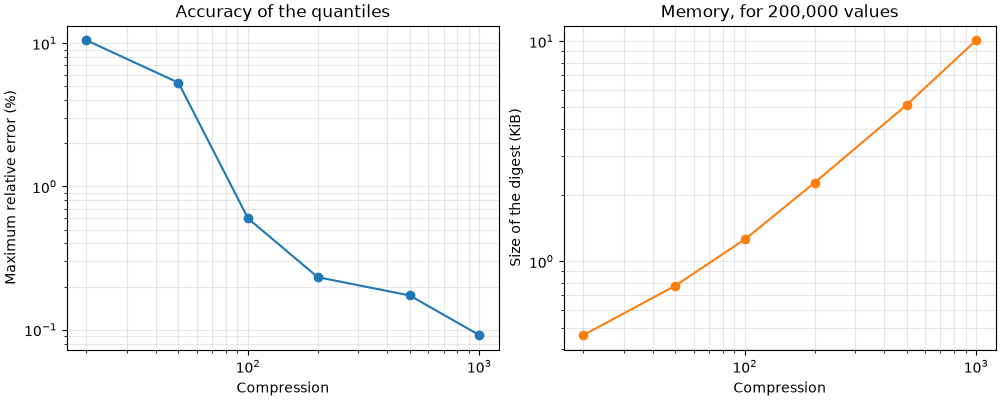
The compression parameter (100 by default) bounds the number of centroids kept by the digest: its size no longer depends on the number of values, only on the compression. Higher values give more accurate quantiles, especially in the tails, at the cost of memory. We measure the size of the digest by its pickled state. The same parameter is accepted by pyinterp.Histogram2D, where it applies to every bin.

compressions = numpy.array([20, 50, 100, 200, 500, 1000])
max_error = []
size_kib = []
for compression in compressions:
    item = pyinterp.TDigest(stream, compression=int(compression))
    max_error.append(
        numpy.abs(item.quantile(probabilities) / exact - 1).max())
    size_kib.append(len(pickle.dumps(item)) / 1024)

fig, (ax1, ax2) = matplotlib.pyplot.subplots(1,
                                             2,
                                             figsize=(10, 4),
                                             layout='constrained')
ax1.loglog(compressions, numpy.array(max_error) * 100, 'o-')
ax1.set_xlabel('Compression')
ax1.set_ylabel('Maximum relative error (%)')
ax1.set_title('Accuracy of the quantiles')
ax1.grid(True, which='both', alpha=0.3)
ax2.loglog(compressions, size_kib, 'o-', color='tab:orange')
ax2.set_xlabel('Compression')
ax2.set_ylabel('Size of the digest (KiB)')
ax2.set_title(f'Memory, for {stream.size:,} values')
ax2.grid(True, which='both', alpha=0.3)