Statistics on Chunked Data with Dask

When a dataset no longer fits in memory, the statistics containers of pyinterp can still be used: the pyinterp.dask helpers process each chunk of a Dask array independently and merge the partial results into a single container. In this example, you will learn how to compute descriptive statistics, quantiles, binned statistics and histograms on chunked arrays, and check that the result matches the in-memory computation.

import dask
import dask.array
import matplotlib.pyplot
import numpy

import pyinterp
import pyinterp.dask

How It Works

Every helper follows the same map then merge pattern:

1. dask.array.map_blocks() builds, for each chunk, a fresh container (e.g. a pyinterp.Binning2D) and feeds it the values of that chunk only. The chunks are processed in parallel by the Dask scheduler.

2. The partial containers are gathered and combined with the += operator, which merges counts, moments, extrema and T-Digest centroids exactly as if all the values had been pushed into a single container.

Only one container per chunk is kept in memory, never the full dataset. Here we use the threaded scheduler so the example runs locally, without a distributed cluster.

dask.config.set(scheduler="threads")

<dask.config.set object at 0x7089256e6850>

Building Chunked Arrays

We generate two million scattered observations of a smooth global field plus some noise. In a real application the arrays would come from files opened lazily (e.g. with xarray.open_mfdataset() or dask.array.from_zarr()); here we wrap NumPy arrays with dask.array.from_array() and split them into chunks of 250,000 points.

rng = numpy.random.default_rng(0)
size = 2_000_000
lon = rng.uniform(-180.0, 180.0, size)
lat = rng.uniform(-80.0, 80.0, size)
field = numpy.cos(numpy.radians(lat)) * numpy.sin(2 * numpy.radians(lon))
values = field + rng.normal(0.0, 0.3, size)

chunks = 250_000
x = dask.array.from_array(lon, chunks=chunks)
y = dask.array.from_array(lat, chunks=chunks)
z = dask.array.from_array(values, chunks=chunks)
print(f"{z.npartitions} chunks of {chunks:,} points")

8 chunks of 250,000 points

Descriptive Statistics

pyinterp.dask.descriptive_statistics() returns the same object as pyinterp.DescriptiveStatistics. Mean, variance, skewness and kurtosis are merged with numerically stable formulas, so the result agrees with the in-memory computation to rounding error.

stats = pyinterp.dask.descriptive_statistics(z)
eager = pyinterp.DescriptiveStatistics(values)
print(f"count={stats.count()}, mean={stats.mean():.6f}, "
      f"std={numpy.sqrt(stats.variance()):.6f}")
for name in ("mean", "variance", "skewness", "kurtosis", "min", "max"):
    numpy.testing.assert_allclose(getattr(stats, name)(),
                                  getattr(eager, name)(),
                                  rtol=1e-10)

count=2000000, mean=0.000097, std=0.609060

Quantiles

pyinterp.dask.tdigest() builds one pyinterp.TDigest per chunk and merges their centroids. The T-Digest is an approximation, so the quantiles are compared with numpy.quantile() using a tolerance rather than an exact equality.

digest = pyinterp.dask.tdigest(z, compression=200)
q = numpy.array([0.01, 0.25, 0.5, 0.75, 0.99])
approx = digest.quantile(q)
exact = numpy.quantile(values, q)
print("Quantiles:", " ".join(f"{v:+.4f}" for v in approx))
print(f"Max abs. difference vs numpy: {numpy.abs(approx - exact).max():.1e}")

Quantiles: -1.2949 -0.4519 -0.0001 +0.4524 +1.2959
Max abs. difference vs numpy: 1.6e-03

Binned Statistics

pyinterp.dask.binning2d() takes a pyinterp.Binning2D that only describes the grid: it is copied internally and left empty. The returned instance holds the statistics accumulated over all the chunks. The simple keyword selects nearest-bin (True) or linear binning.

binning = pyinterp.Binning2D(
    pyinterp.Axis(numpy.arange(-180.0, 180.0, 5.0), period=360.0),
    pyinterp.Axis(numpy.arange(-80.0, 80.1, 5.0)),
)
binned = pyinterp.dask.binning2d(x, y, z, binning, simple=True)
print(f"Template still empty: {binning.count().sum() == 0}")

Template still empty: True

Pushing the same data into the template in a single call gives the reference result. The two grids agree to rounding error, since only the order of the additions differs.

binning.push(lon, lat, values, simple=True)
numpy.testing.assert_array_equal(binned.count(), binning.count())
diff = numpy.nanmax(numpy.abs(binned.mean() - binning.mean()))
print(f"Max abs. difference of the binned mean: {diff:.1e}")

Max abs. difference of the binned mean: 0.0e+00

Histograms

pyinterp.dask.histogram2d() works the same way with a pyinterp.Histogram2D, which keeps a compressed histogram in each bin and therefore gives access to quantiles such as the median. Like the T-Digest, merging histograms is approximate for quantiles, but exact for counts, means and extrema.

histogram = pyinterp.Histogram2D(
    pyinterp.Axis(numpy.arange(-180.0, 180.0, 5.0), period=360.0),
    pyinterp.Axis(numpy.arange(-80.0, 80.1, 5.0)),
)
hist = pyinterp.dask.histogram2d(x, y, z, histogram)
median = hist.quantile(0.5)
histogram.push(lon, lat, values)
numpy.testing.assert_array_equal(hist.count(), histogram.count())
diff = numpy.nanmax(numpy.abs(median - histogram.quantile(0.5)))
print(f"Max abs. difference of the binned median: {diff:.1e}")

Max abs. difference of the binned median: 0.0e+00

Visualizing the Results

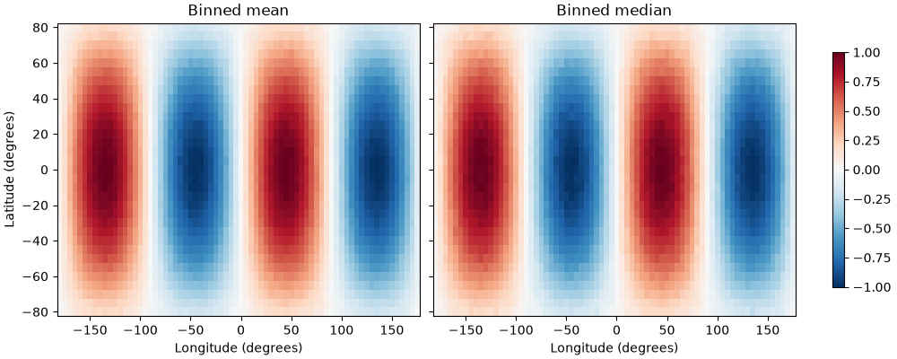
The mean computed by pyinterp.dask.binning2d() and the median computed by pyinterp.dask.histogram2d() both recover the underlying field from the noisy observations.

lon_grid = binned.x[:]
lat_grid = binned.y[:]
fig, axes = matplotlib.pyplot.subplots(1,
                                       2,
                                       figsize=(10, 4),
                                       layout="constrained",
                                       sharey=True)
for ax, data, title in zip(axes, (binned.mean(), median),
                           ("Binned mean", "Binned median"),
                           strict=True):
    pcm = ax.pcolormesh(lon_grid,
                        lat_grid,
                        data.T,
                        cmap="RdBu_r",
                        vmin=-1,
                        vmax=1,
                        shading="auto")
    ax.set_title(title)
    ax.set_xlabel("Longitude (degrees)")
axes[0].set_ylabel("Latitude (degrees)")
fig.colorbar(pcm, ax=axes, shrink=0.8)
matplotlib.pyplot.show()

See also

Binning explains the difference between simple and linear binning, and Descriptive Statistics details the statistics available on pyinterp.DescriptiveStatistics.