Binning on the Sphere

The Binning example bins data on a grid whose cells are treated as flat rectangles. When the grid is defined in longitude and latitude, this approximation degrades towards the poles, where the cells shrink and are no longer symmetric about their center. This example shows how to give pyinterp.Binning2D() a spheroid so that linear binning computes its weights from geodetic areas, how to merge partial binnings with +=, and how to compute a weighted 1D profile with pyinterp.Binning1D().

import matplotlib.pyplot
import numpy

import pyinterp
from pyinterp.geometry import geographic

Bilinear Weights on the Ellipsoid

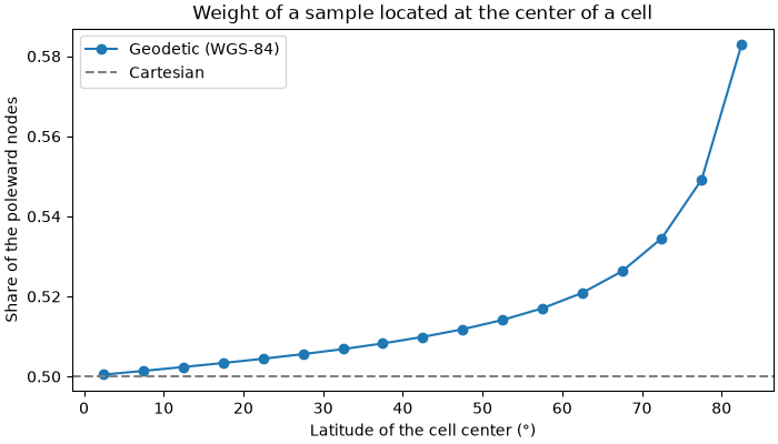
With linear binning, each sample is spread over the four nodes surrounding it: the weight of a node is the area of the sub-cell opposite to it, divided by the area of the whole cell. Without a spheroid, these areas are computed in the plane, so a sample located at the center of a cell always gives a weight of 0.25 to each node. With a pyinterp.geometry.geographic.Spheroid (WGS-84 by default), the areas are measured on the ellipsoid. Because the poleward half of a cell is smaller than its equatorward half, the two poleward nodes receive more weight.

We push one sample at the center of a 10° x 5° cell, for cells located at increasing latitudes, and read back the weight given to each node with sum_of_weights.

wgs84 = geographic.Spheroid()
latitudes = numpy.arange(0.0, 85.0, 5.0)
poleward = []
for lat in latitudes:
    cell = pyinterp.Binning2D(
        pyinterp.Axis(numpy.array([0.0, 10.0])),
        pyinterp.Axis(numpy.array([lat, lat + 5.0])),
        spheroid=wgs84,
    )
    cell.push(
        numpy.array([5.0]),
        numpy.array([lat + 2.5]),
        numpy.array([1.0]),
        simple=False,
    )
    weights = cell.sum_of_weights()
    # Column 1 holds the two nodes located on the poleward edge.
    poleward.append(weights[:, 1].sum() / weights.sum())

fig, ax = matplotlib.pyplot.subplots(figsize=(7, 4), layout="constrained")
ax.plot(latitudes + 2.5, poleward, "o-", label="Geodetic (WGS-84)")
ax.axhline(0.5, color="gray", linestyle="--", label="Cartesian")
ax.set_xlabel("Latitude of the cell center (°)")
ax.set_ylabel("Share of the poleward nodes")
ax.set_title("Weight of a sample located at the center of a cell")
ax.legend()

<matplotlib.legend.Legend object at 0x7c4010a44ad0>

Synthetic Data at High Latitude

We sample a smooth field at random positions uniformly distributed over the sphere between 60°N and 85°N. The field mostly varies with latitude, with a weak zonal wave and some measurement noise.

rng = numpy.random.default_rng(0)
size = 200_000
lon = rng.uniform(-40.0, 40.0, size)
lat = numpy.degrees(
    numpy.arcsin(
        rng.uniform(numpy.sin(numpy.radians(60.0)),
                    numpy.sin(numpy.radians(85.0)), size)))
truth = lat + 2.0 * numpy.cos(numpy.radians(9.0 * lon))
values = truth + rng.normal(0.0, 0.5, size)

Simple and Linear Binning

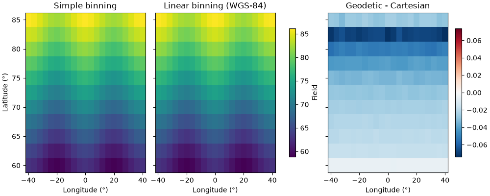
We build two binnings on the same 4° x 2.5° grid: one without spheroid (Cartesian weights) and one with WGS-84. Simple binning only assigns each sample to its nearest node, so it ignores the spheroid; the difference only appears with linear binning.

x_axis = pyinterp.Axis(numpy.arange(-40.0, 40.1, 4.0), period=360.0)
y_axis = pyinterp.Axis(numpy.arange(60.0, 85.1, 2.5))

cartesian = pyinterp.Binning2D(x_axis, y_axis)
geodetic = pyinterp.Binning2D(x_axis, y_axis, spheroid=wgs84)

cartesian.push(lon, lat, values, simple=True)
simple_mean = cartesian.mean()

cartesian.clear()
cartesian.push(lon, lat, values, simple=False)
geodetic.push(lon, lat, values, simple=False)
linear_mean = geodetic.mean()
delta = geodetic.mean() - cartesian.mean()

The geodetic weights shift each node’s mean towards samples located on the equatorward side of the node, which lowers the latitude-dependent field by a small but systematic amount. The effect grows with latitude, as cells become more asymmetric. Neither set of weights removes the bias of the edge rows (60°N and 85°N), which only receive samples from one side.

mx, my = numpy.meshgrid(x_axis[:], y_axis[:], indexing="ij")
fig, axes = matplotlib.pyplot.subplots(1,
                                       3,
                                       figsize=(10, 4),
                                       layout="constrained",
                                       sharey=True)
for ax, data, title in zip(axes[:2], (simple_mean, linear_mean),
                           ("Simple binning", "Linear binning (WGS-84)")):
    pcm = ax.pcolormesh(mx, my, data, cmap="viridis", shading="auto")
    ax.set_title(title)
fig.colorbar(pcm, ax=axes[:2], shrink=0.8, label="Field")
limit = numpy.nanmax(numpy.abs(delta))
pcm = axes[2].pcolormesh(mx,
                         my,
                         delta,
                         cmap="RdBu_r",
                         shading="auto",
                         vmin=-limit,
                         vmax=limit)
axes[2].set_title("Geodetic - Cartesian")
fig.colorbar(pcm, ax=axes[2], shrink=0.8)
axes[0].set_ylabel("Latitude (°)")
for ax in axes:
    ax.set_xlabel("Longitude (°)")

Merging Binnings

Binning containers can be filled in several batches and combined with +=, for instance when the data are processed in chunks or in parallel (see pyinterp.dask.binning2d()). Here, we bin the two halves of the dataset separately and check that merging them gives the same statistics as binning all the samples at once. Both binnings must share the same axes and the same spheroid, otherwise += raises a ValueError.

half = size // 2
first = pyinterp.Binning2D(x_axis, y_axis, spheroid=wgs84)
second = pyinterp.Binning2D(x_axis, y_axis, spheroid=wgs84)
first.push(lon[:half], lat[:half], values[:half], simple=False)
second.push(lon[half:], lat[half:], values[half:], simple=False)
first += second

print("Same mean:", numpy.allclose(first.mean(), geodetic.mean()))
print("Same variance:",
      numpy.allclose(first.variance(), geodetic.variance()))
print("Same weights:",
      numpy.allclose(first.sum_of_weights(), geodetic.sum_of_weights()))

try:
    first += cartesian
except ValueError as error:
    print("Merging with a Cartesian binning fails:", error)

Same mean: True
Same variance: True
Same weights: True
Merging with a Cartesian binning fails: Cannot combine grids with different geodetic systems

Weighted 1D Binning

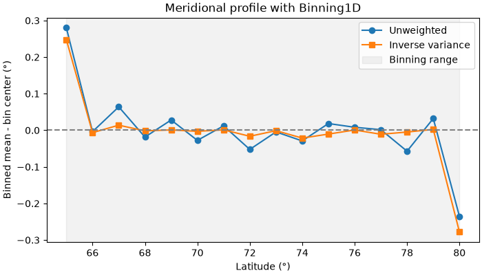
pyinterp.Binning1D() groups samples along a single axis. Its range argument restricts the samples taken into account, and push accepts one weight per sample. We compute a meridional profile of the latitude between 65°N and 80°N, where half of the samples come from a noisy instrument. Weighting each sample by the inverse of its noise variance limits the influence of the noisy ones.

sigma = numpy.where(rng.random(size) < 0.5, 0.5, 5.0)
noisy = lat + rng.normal(0.0, sigma)

profile_axis = pyinterp.Axis(numpy.arange(60.0, 85.1, 1.0))
unweighted = pyinterp.Binning1D(profile_axis, range=(65.0, 80.0))
weighted = pyinterp.Binning1D(profile_axis, range=(65.0, 80.0))
unweighted.push(lat, noisy)
weighted.push(lat, noisy, weights=1.0 / sigma**2)

We plot the error of each profile with respect to the bin centers. The bins at 65°N and 80°N are biased because range discards the samples falling in their outer half.

centers = profile_axis[:]
fig, ax = matplotlib.pyplot.subplots(figsize=(7, 4), layout="constrained")
ax.plot(centers, unweighted.mean() - centers, "o-", label="Unweighted")
ax.plot(centers, weighted.mean() - centers, "s-", label="Inverse variance")
ax.axhline(0.0, color="gray", linestyle="--")
ax.axvspan(65.0, 80.0, color="gray", alpha=0.1, label="Binning range")
ax.set_xlabel("Latitude (°)")
ax.set_ylabel("Binned mean - bin center (°)")
ax.set_title("Meridional profile with Binning1D")
ax.legend()

<matplotlib.legend.Legend object at 0x7c4010ba0c20>