Interpolating an xarray DataArray

pyinterp.backends.xarray.RegularGridInterpolator is the one-call entry point to interpolate a 2-, 3- or 4-D xarray.DataArray: it identifies the axes, builds the matching grid and dispatches to the bivariate, trivariate or quadrivariate interpolator. In this example you will learn how to build it, query it with a dictionary of coordinates (including dates), choose and tune the interpolation method, and what happens at the dateline and outside the grid.

import matplotlib.pyplot
import numpy
import xarray

import pyinterp
import pyinterp.backends.xarray
import pyinterp.tests

Building the Interpolator

We load a global grid of mean sea surface (MSS). The variable is stored as (lat, lon), but the interpolator does not care about the order of the dimensions: the longitude and latitude are recognized from the units attribute of their coordinates (degrees_east and degrees_north, see pyinterp.cf.AxisLongitudeUnit and pyinterp.cf.AxisLatitudeUnit), and the data is transposed to (longitude, latitude) internally.

ds = pyinterp.tests.load_grid2d()
interpolator = pyinterp.backends.xarray.RegularGridInterpolator(ds.mss)
print(f"dims={ds.mss.dims}, ndim={interpolator.ndim}")
print(interpolator.grid)

dims=('lat', 'lon'), ndim=2
Grid2D(shape=(1440, 712), dtype=float64, nbytes=7 MB)

Querying with a Dictionary of Coordinates

The interpolator is called with a dictionary that maps every dimension name to the coordinates of the points to evaluate. The values can be scalars, lists or arrays of any shape: they are broadcast against each other, and the result has their broadcast shape, here the shape of the 2-D target grid. The MSS is stored with longitudes in [0, 360), but we query it in [-180, 180).

mx, my = numpy.meshgrid(
    numpy.arange(-180, 180, 1.0) + 1 / 3,
    numpy.arange(-80, 80, 1.0) + 1 / 3,
    indexing="ij",
)
coords = {"lon": mx, "lat": my}
bilinear = interpolator(coords)

Choosing the Method

The method argument selects the interpolator. bilinear (default), nearest and idw only use the cell surrounding the point. Windowed methods (bicubic, c_spline, akima, steffen…) fit a function on a window of neighboring nodes; its size is set by half_window_size_x and half_window_size_y, and boundary_mode decides whether the window may shrink near the edges of the grid ("shrink") or whether the result is undefined there ("undef", the default). The other keyword arguments, such as num_threads, are forwarded to pyinterp.bivariate().

bicubic = interpolator(
    coords,
    method="bicubic",
    half_window_size_x=3,
    half_window_size_y=3,
    boundary_mode="shrink",
)

The two methods agree to within a millimeter; the largest differences follow the strongest gradients of the field. Note that a window containing a single masked (NaN) node gives NaN, so the windowed method loses a few points along the coasts.

print(
    f"NaN: bilinear={numpy.isnan(bilinear).sum()}, "
    f"bicubic={numpy.isnan(bicubic).sum()}"
)
fig, (ax1, ax2) = matplotlib.pyplot.subplots(
    2, 1, figsize=(10, 6), sharex=True, layout="constrained"
)
pcm = ax1.pcolormesh(mx, my, bilinear, cmap="viridis", vmin=-0.1, vmax=0.1)
fig.colorbar(pcm, ax=ax1, label="MSS (m)")
ax1.set_title("Bilinear interpolation, longitudes in [-180, 180)")
pcm = ax2.pcolormesh(
    mx, my, (bicubic - bilinear) * 1e3, cmap="RdBu_r", vmin=-0.5, vmax=0.5
)
fig.colorbar(pcm, ax=ax2, label="mm")
ax2.set_title("Bicubic minus bilinear")
ax2.set_xlabel("Longitude (degrees)")
for ax in (ax1, ax2):
    ax.set_ylabel("Latitude (degrees)")

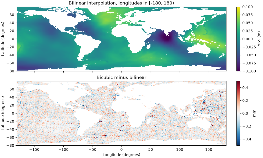
NaN: bilinear=19133, bicubic=21880

Longitude Periodicity

A longitude axis is always created as periodic (360 degrees). Longitudes are therefore never out of bounds: the same location written as -0.1, 359.9 or 719.9 degrees gives the same value, and points between the last column (359.75) and 360 are interpolated across the seam of the grid.

print(interpolator({"lon": [-0.1, 359.9, 719.9], "lat": -40.1}))

[0.017 0.017 0.017]

Outside the Grid

The latitudes cover [-89, 88.75]. A point beyond this range returns NaN by default; set bounds_error=True to raise a ValueError instead.

outside = {"lon": -30.0, "lat": 89.5}
print(interpolator(outside))
try:
    interpolator(outside, bounds_error=True)
except ValueError as exc:
    print(f"ValueError: {exc}")

nan
ValueError: 89.5 is out of bounds for axis y [-89, ..., 88.75]

Adding a Time Dimension

With a 3-D array the interpolator becomes trivariate. Here the total column water vapor is stored as (time, latitude, longitude) with daily values. A coordinate of type datetime64 is detected as a temporal axis and moved to the third position, so the query dates are simply passed as datetime64 values, at any resolution.

tcw = pyinterp.tests.load_grid3d().tcw
interpolator = pyinterp.backends.xarray.RegularGridInterpolator(tcw)
print(interpolator.grid)

dates = numpy.arange(
    numpy.datetime64("2002-07-02T00", "h"),
    numpy.datetime64("2002-07-12T00", "h"),
    numpy.timedelta64(3, "h"),
)
track = {
    "longitude": 10.3,
    "latitude": 45.1,
    "time": dates,
}

TemporalGrid3D(shape=(144, 73, 31), dtype=float64, nbytes=2 MB)

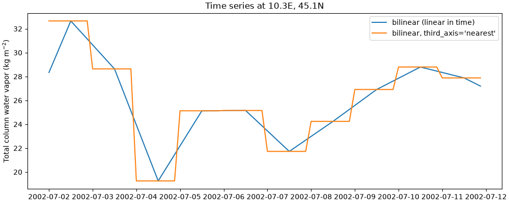
The default bilinear method is linear along the time axis. The third_axis option ("linear" or "nearest") selects the interpolation along time; for a 4-D array, fourth_axis plays the same role for the fourth dimension. These options, like half_window_size_x, select the windowed version of bilinear.

linear = interpolator(track)
nearest = interpolator(track, method="bilinear", third_axis="nearest")

fig, ax = matplotlib.pyplot.subplots(figsize=(10, 4), layout="constrained")
ax.plot(dates, linear, label="bilinear (linear in time)")
ax.plot(dates, nearest, label="bilinear, third_axis='nearest'")
ax.set_ylabel("Total column water vapor (kg m$^{-2}$)")
ax.set_title("Time series at 10.3E, 45.1N")
ax.legend()

<matplotlib.legend.Legend object at 0x7d1144822e40>

A 4-D array works the same way: with (time, level, latitude, longitude) dimensions, the axes are reordered to (longitude, latitude, time, level), and the dictionary must name all four dimensions.

pressure = pyinterp.tests.load_grid4d().pressure
interpolator = pyinterp.backends.xarray.RegularGridInterpolator(pressure)
print(interpolator.grid)

TemporalGrid4D(shape=(12, 6, 2, 2), dtype=float32, nbytes=1 KB)

Labelled Results with the pyinterp Accessor

Once pyinterp and xarray are imported, data arrays and datasets have a pyinterp accessor. Its interp() method follows xarray.DataArray.interp(): the coordinates are passed as keyword arguments, and the result is a DataArray labelled with them, which keeps the name and the attributes of the variable. One-dimensional coordinates define a new grid, so there is no meshgrid to build.

mss = ds.mss.pyinterp.interp(
    lon=numpy.arange(-180, 180, 0.5),
    lat=numpy.arange(-80, 80, 0.5),
    method="bicubic",
)
print(mss)

<xarray.DataArray 'mss' (lat: 320, lon: 720)> Size: 2MB
array([[  nan,   nan,   nan, ...,   nan,   nan,   nan],
       [  nan,   nan,   nan, ...,   nan,   nan,   nan],
       [  nan,   nan,   nan, ...,   nan,   nan,   nan],
       ...,
       [0.002, 0.002, 0.002, ..., 0.001, 0.002, 0.002],
       [0.002, 0.002, 0.002, ..., 0.002, 0.002, 0.002],
       [0.002, 0.002, 0.002, ..., 0.002, 0.002, 0.002]], shape=(320, 720))
Coordinates:
  * lat      (lat) float64 3kB -80.0 -79.5 -79.0 -78.5 ... 78.0 78.5 79.0 79.5
  * lon      (lon) float64 6kB -180.0 -179.5 -179.0 -178.5 ... 178.5 179.0 179.5
Attributes:
    long_name:     Mean sea surface height above reference ellipsoid
    units:         m
    grid_mapping:  crs
    source:        SMO15_1s60_V2.dat
    cell_methods:  lon: point lat: point

Coordinates given as data arrays sharing a dimension are interpolated point by point, along a track for instance. The keyword arguments that do not name a dimension are the options of the interpolator, and dates can be given as strings.

track = tcw.pyinterp.interp(
    longitude=xarray.DataArray(numpy.linspace(-30, 30, 50), dims="obs"),
    latitude=xarray.DataArray(numpy.linspace(-20, 40, 50), dims="obs"),
    time="2002-07-05T12:00",
    bounds_error=True,
)
print(track)

<xarray.DataArray 'tcw' (obs: 50)> Size: 400B
array([24.47455481, 27.78406211, 30.50603547, 25.12550513, 19.3178315 ,
       25.70561549, 32.64532029, 35.09478524, 36.64133985, 37.316209  ,
       37.92638815, 37.06678047, 35.08439326, 33.29223999, 31.53000256,
       31.32761604, 31.54333934, 34.86044902, 39.56814296, 43.9054787 ,
       49.14237962, 52.02903909, 52.62723436, 52.20315115, 50.58550299,
       49.70437078, 49.69870273, 48.10531923, 45.46202381, 42.17753016,
       38.70367639, 32.1830379 , 20.17924025, 14.31828244, 12.80989271,
       11.3287591 , 14.6402907 , 18.40654166, 20.3557168 , 21.63105744,
       23.3943745 , 23.74053944, 23.09037355, 22.39021747, 22.59515799,
       22.1344152 , 20.58533696, 18.52913462, 17.40691458, 18.09264074])
Coordinates:
    latitude   (obs) float64 400B -20.0 -18.78 -17.55 ... 37.55 38.78 40.0
    longitude  (obs) float64 400B -30.0 -28.78 -27.55 ... 27.55 28.78 30.0
    time       datetime64[ns] 8B 2002-07-05T12:00:00
Dimensions without coordinates: obs
Attributes:
    units:      kg m**-2
    long_name:  Total column water

When to Use It

The pyinterp accessor is the shortest path when the data is already an xarray.DataArray and a labelled result is wanted; it builds the grid at each call, so keep a RegularGridInterpolator to interpolate the same variable many times. The interpolator is one class for any number of dimensions, coordinates passed by name, dates handled for you. It is a thin wrapper around Grid2D, Grid3D and Grid4D; use these classes and their bivariate, trivariate or quadrivariate methods, or build a pyinterp.Grid and call pyinterp.bivariate() and friends, when you work with plain numpy arrays, need full control over the axes (a non-periodic longitude, for instance), or reuse a configuration object. These lower-level interfaces are shown in 2D Interpolation, 3D Interpolation and 4D Interpolation.