1D Interpolation

This example illustrates how to perform 1D interpolation of a variable on a regular grid. The pyinterp library provides several interpolation methods for univariate data, including linear and various spline-based approaches.

import matplotlib.pyplot
import numpy

import pyinterp

Linear Interpolation

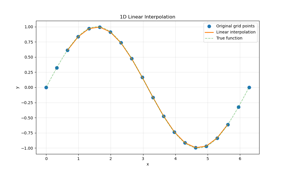
Linear interpolation is the simplest method for estimating values between grid points. In this section, we will perform linear interpolation on a 1D grid using pyinterp.

First, let’s create a simple 1D grid with a sine wave function.

x_grid = numpy.linspace(0, 2 * numpy.pi, 20)
y_grid = numpy.sin(x_grid)

Create the interpolator using the Grid class. We need to create an Axis object for the x-coordinates and then build the grid.

x_axis = pyinterp.core.Axis(x_grid)
grid = pyinterp.core.Grid(x_axis, y_grid)

Now, let’s define the coordinates where we want to interpolate the grid. We’ll create a finer grid to see the interpolation result.

x_interp = numpy.linspace(0, 2 * numpy.pi, 200)

Perform linear interpolation using the univariate function.

y_linear = pyinterp.univariate(grid, x_interp, method="linear")

Let’s visualize the original grid points and the interpolated values.

fig, ax = matplotlib.pyplot.subplots(figsize=(10, 6))
ax.plot(x_grid, y_grid, "o", label="Original grid points", markersize=8)
ax.plot(x_interp, y_linear, "-", label="Linear interpolation", linewidth=2)
ax.plot(x_interp, numpy.sin(x_interp), "--", label="True function", alpha=0.5)
ax.set_xlabel("x")
ax.set_ylabel("y")
ax.set_title("1D Linear Interpolation")
ax.legend()
ax.grid(True, alpha=0.3)

Spline Interpolation

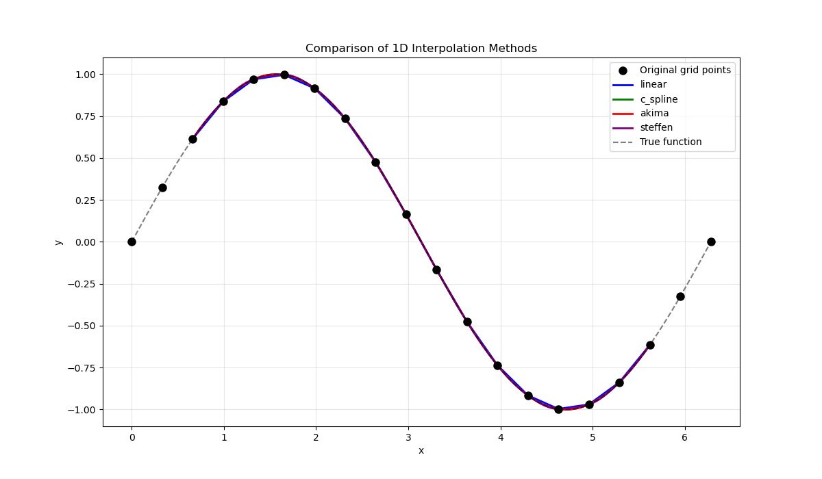
Spline interpolation provides smoother results compared to linear interpolation by using polynomial curves. The library supports several spline methods.

The univariate method supports multiple interpolation techniques:

• linear: Linear interpolation between grid points

• polynomial: Polynomial interpolation

• c_spline: Cubic spline with natural boundary conditions

• c_spline_periodic: Cubic spline with periodic boundary conditions

• akima: Akima spline (avoids overshooting)

• akima_periodic: Akima spline with periodic boundary conditions

• steffen: Steffen spline (monotonic interpolation)

Let’s compare different interpolation methods.

methods = ["linear", "c_spline", "akima", "steffen"]
colors = ["blue", "green", "red", "purple"]

fig, ax = matplotlib.pyplot.subplots(figsize=(12, 7))
ax.plot(
    x_grid, y_grid, "ko", label="Original grid points", markersize=8, zorder=5
)

for method, color in zip(methods, colors, strict=False):
    y_interp = pyinterp.univariate(grid, x_interp, method=method)
    ax.plot(
        x_interp, y_interp, "-", label=f"{method}", color=color, linewidth=2
    )

ax.plot(
    x_interp,
    numpy.sin(x_interp),
    "k--",
    label="True function",
    alpha=0.5,
    linewidth=1.5,
)
ax.set_xlabel("x")
ax.set_ylabel("y")
ax.set_title("Comparison of 1D Interpolation Methods")
ax.legend()
ax.grid(True, alpha=0.3)

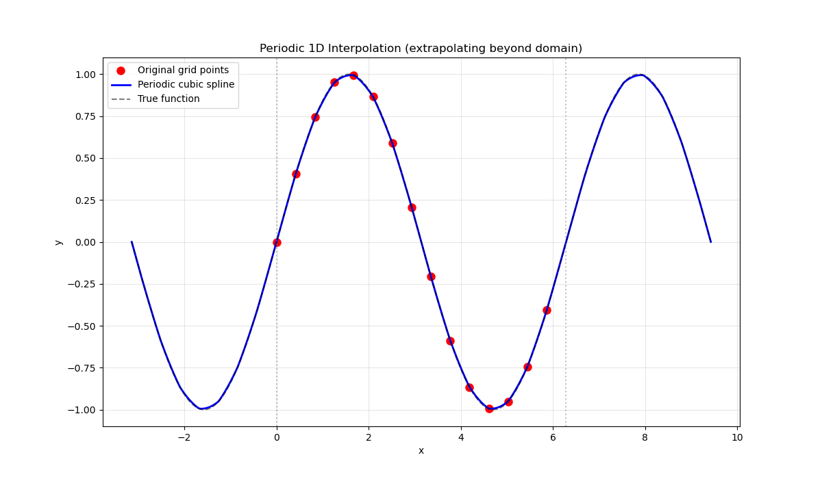
Interpolation with Periodic Boundary Conditions

For periodic data (like angles or cyclic phenomena), we can use periodic spline methods or create an axis with a defined period.

Let’s create a periodic grid and compare periodic vs non-periodic interpolation.

x_periodic = numpy.linspace(0, 2 * numpy.pi, 15, endpoint=False)
y_periodic = numpy.sin(x_periodic)

# Create periodic axis
x_axis_periodic = pyinterp.core.Axis(x_periodic, period=2 * numpy.pi)
grid_periodic = pyinterp.core.Grid(x_axis_periodic, y_periodic)

# Interpolate beyond the original domain to see the periodic effect
x_extended = numpy.linspace(-numpy.pi, 3 * numpy.pi, 400)

y_periodic_interp = pyinterp.univariate(
    grid_periodic, x_extended, method="c_spline_periodic"
)

Visualize the periodic interpolation.

fig, ax = matplotlib.pyplot.subplots(figsize=(12, 7))
ax.plot(
    x_periodic, y_periodic, "ro", label="Original grid points", markersize=8
)
ax.plot(
    x_extended,
    y_periodic_interp,
    "b-",
    label="Periodic cubic spline",
    linewidth=2,
)
ax.plot(
    x_extended, numpy.sin(x_extended), "k--", label="True function", alpha=0.5
)
ax.axvline(x=0, color="gray", linestyle=":", alpha=0.5)
ax.axvline(x=2 * numpy.pi, color="gray", linestyle=":", alpha=0.5)
ax.set_xlabel("x")
ax.set_ylabel("y")
ax.set_title("Periodic 1D Interpolation (extrapolating beyond domain)")
ax.legend()
ax.grid(True, alpha=0.3)

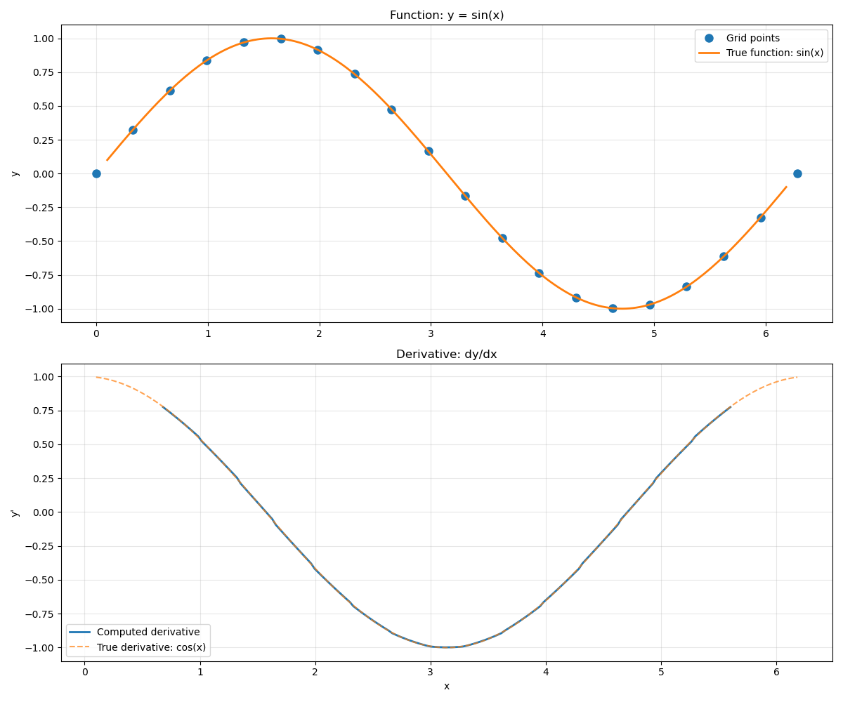
Computing Derivatives

The library also supports computing derivatives of the interpolated function using the univariate_derivative function.

Let’s compute and compare the derivative of our sine function. The analytical derivative is cos(x).

x_deriv = numpy.linspace(0.1, 2 * numpy.pi - 0.1, 200)

derivative = pyinterp.univariate_derivative(grid, x_deriv, method="c_spline")

Visualize the derivative.

fig, (ax1, ax2) = matplotlib.pyplot.subplots(2, 1, figsize=(12, 10))

# Plot function
ax1.plot(x_grid, y_grid, "o", label="Grid points", markersize=8)
ax1.plot(
    x_deriv,
    numpy.sin(x_deriv),
    "-",
    label="True function: sin(x)",
    linewidth=2,
)
ax1.set_ylabel("y")
ax1.set_title("Function: y = sin(x)")
ax1.legend()
ax1.grid(True, alpha=0.3)

# Plot derivative
ax2.plot(x_deriv, derivative, "-", label="Computed derivative", linewidth=2)
ax2.plot(
    x_deriv,
    numpy.cos(x_deriv),
    "--",
    label="True derivative: cos(x)",
    alpha=0.7,
)
ax2.set_xlabel("x")
ax2.set_ylabel("y'")
ax2.set_title("Derivative: dy/dx")
ax2.legend()
ax2.grid(True, alpha=0.3)

matplotlib.pyplot.tight_layout()

Advanced Options

The univariate interpolation method accepts additional parameters to control the interpolation window size and boundary handling.

Note

When using spline interpolation methods, the behavior near grid edges is controlled by the boundary_mode parameter. Two modes are available:

• undef (Undefined Boundary) - Default: The interpolation window must fit entirely within the grid. If a query point is too close to the edge and the full window cannot be extracted, the interpolation returns NaN.

• shrink (Shrink Boundary): The interpolation window adaptively shrinks at grid boundaries to use available data. This allows interpolation closer to edges but may affect smoothness in those regions.

Let’s demonstrate the boundary mode effect.

x_edge = numpy.array([0.05, 0.1, 2 * numpy.pi - 0.1, 2 * numpy.pi - 0.05])

# With default boundary mode (undef)
y_undef = pyinterp.univariate(grid, x_edge, method="c_spline")

# With shrink boundary mode
y_shrink = pyinterp.univariate(
    grid, x_edge, method="c_spline", boundary_mode="shrink"
)

print("Interpolation near boundaries:")
print(f"x coordinates: {x_edge}")
print(f"Undef mode:    {y_undef}")
print(f"Shrink mode:   {y_shrink}")
print(f"True values:   {numpy.sin(x_edge)}")

Interpolation near boundaries:
x coordinates: [0.05       0.1        6.18318531 6.23318531]
Undef mode:    [nan nan nan nan]
Shrink mode:   [ 0.04982433  0.09954609 -0.09954609 -0.04982433]
True values:   [ 0.04997917  0.09983342 -0.09983342 -0.04997917]