Reduced Gaussian Grids

ECMWF distributes its analyses and forecasts on reduced Gaussian grids: a fixed set of parallels, the Gaussian latitudes, each holding equally spaced points whose number decreases towards the poles. pyinterp.reduced_gaussian interpolates them in 2D, in 3D (a column of model levels per point) and in time, from numeric inputs only: the latitudes of the parallels, their number of points and the values. In this example you will learn how to describe the mesh, read only the part of a grid a pass needs, interpolate a series of 2D and 3D grids along a satellite pass, and compute corrections from the interpolated columns, with numpy or with a function compiled by numba. The last section gives the same workflow on GRIB files read with ecCodes.

The data are a subset of the operational ECMWF N640 analyses of 2018-02-13 at 12h and 18h, in a box across the Greenwich meridian (4°W to 4°E, 42°N to 48°N): the surface pressure, and the temperature and the specific humidity on 9 of the 137 model levels.

import importlib.util

import matplotlib.pyplot
import numpy

import pyinterp.tests
from pyinterp import reduced_gaussian as rg


ds = pyinterp.tests.load_reduced_gaussian()

The Mesh

The Mesh is the geometry alone: the latitudes of the parallels, north to south, and their number of points. The points are numbered parallel after parallel from the north, and on each parallel eastwards from longitude 0, as a global GRIB field stores them. gaussian_latitudes() and octahedral_points() build the standard meshes when no file is at hand.

mesh = rg.Mesh(ds.latitude.values, ds.pl.values)
print(f"{mesh.ny} parallels, {mesh.size} points")

fig, ax = matplotlib.pyplot.subplots(figsize=(8, 4), layout="constrained")
ax.plot(mesh.latitudes, mesh.points_per_parallel, label="N640 (this grid)")
octahedral = rg.octahedral_points(640)
ax.plot(rg.gaussian_latitudes(640), octahedral, label="O640 (octahedral)")
ax.set_xlabel("Latitude (degrees)")
ax.set_ylabel("Points per parallel")
ax.legend()

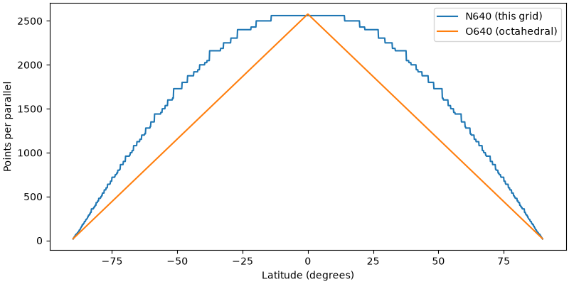
1280 parallels, 2140702 points

<matplotlib.legend.Legend object at 0x7d1144822270>

Reading Only a Zone

A global N640 field holds 2.1 million points per level. A Zone is the part of the mesh a regional grid holds: sorted ranges [start, stop) of the flat indices of the mesh, computed from the mesh alone, before any value is read. The dataset stores the zone of its box; Zone.from_box computes it again from the box, given unwrapped across the Greenwich meridian.

box = rg.Zone.from_box(mesh, -4.0, 42.0, 4.0, 48.0)
assert box == rg.Zone(mesh, ds.ranges.values)
print(f"Box: {box.size} points in {box.num_ranges} ranges")

Box: 1904 points in 45 ranges

For a satellite pass, Zone.from_points holds exactly the corners the points read: a pass is a thin line, far smaller than its bounding box. The pass below crosses the box in one hour, between the two analyses.

s = numpy.linspace(0.0, 1.0, 3600)
lon = -3.5 + 7.0 * s
lat = 42.5 + 5.0 * s
dates = numpy.datetime64("2018-02-13T13", "ns") + (s * 3600e9).astype("m8[ns]")
track = rg.Zone.from_points(mesh, lon, lat)
print(f"Pass: {track.size} points in {track.num_ranges} ranges")

Pass: 146 points in 39 ranges

The values of a zone are read with its indices(), which index a NumPy array or make an orthogonal selection in a Zarr or netCDF variable, or with its ranges() for readers that seek in a file. Many small reads cost more than a few larger ones: coalesce() merges the ranges closer than a gap, and gives the positions of the values of the zone in what was read. The pass reads a few points per parallel, about 2000 points apart on these parallels: a gap of 5000 points reads the zone at once.

for io_gap in (0, 1000, 5000):
    merged, gather = rg.coalesce(track.ranges(), io_gap)
    read = int((merged[:, 1] - merged[:, 0]).sum())
    print(f"io_gap={io_gap:5d}: {len(merged):3d} reads, {read:5d} points read")

io_gap=    0:  39 reads,   146 points read
io_gap= 1000:  39 reads,   146 points read
io_gap= 5000:   1 reads, 70841 points read

Here the dataset holds the values of the box. The values of the pass are those of the box at the indices of the pass: a zone maps a flat index of the mesh to the row of its values.

rows = box.rows(track.indices())
assert numpy.all(rows >= 0)

A Series of 2D Grids

A Grid holds the fields of one time step, on the mesh or on a zone: float32 or float64 arrays of shape (points,), read without copy. A Series holds the steps. Each step may hold its own zone, which time_zones() computes from the points whose date reads the step.

zones = rg.time_zones(mesh, ds.time.values, dates, lon, lat)
surface = rg.Series(mesh)
for k, (time, zone) in enumerate(zip(ds.time.values, zones, strict=True)):
    sp = ds.sp.values[k][box.rows(zone.indices())]
    surface.append(time, rg.Grid(mesh, {"sp": sp}, zone=zone))
    print(f"{time}: {zone.size} points")

2018-02-13T12:00:00.000000000: 146 points
2018-02-13T18:00:00.000000000: 146 points

interpolate() locates each point once on the mesh, interpolates the two analyses that bracket its date on the trapezoidal cell around it, and blends them in time.

sp = rg.interpolate(surface, lon, lat, dates)["sp"]
at12, at18 = (
    rg.interpolate(surface, lon, lat, numpy.full(lon.size, time))["sp"]
    for time in ds.time.values
)
nearest = rg.interpolate(surface, lon, lat, dates, time_method="nearest")

fig, ax = matplotlib.pyplot.subplots(figsize=(8, 4), layout="constrained")
ax.plot(lat, at12 / 100, ":", label="12h analysis")
ax.plot(lat, at18 / 100, ":", label="18h analysis")
ax.plot(lat, sp / 100, label="13h-14h, linear in time")
ax.plot(lat, nearest["sp"] / 100, "--", label="nearest in time")
ax.set_xlabel("Latitude of the pass (degrees)")
ax.set_ylabel("Surface pressure (hPa)")
ax.legend()

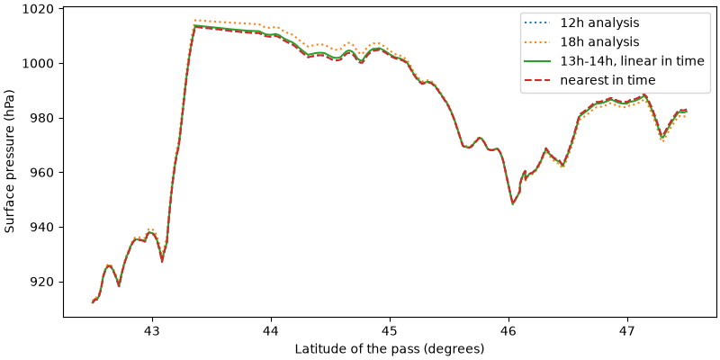
<matplotlib.legend.Legend object at 0x7d11448ec2f0>

A computation point by point from 2D fields needs nothing more than NumPy: here the dry tropospheric correction from the surface pressure.

dry = -2.277e-5 * sp * (1.0 + 0.0026 * numpy.cos(numpy.radians(2.0 * lat)))
print(f"Dry tropospheric correction: {dry.min():.3f} to {dry.max():.3f} m")

Dry tropospheric correction: -2.309 to -2.078 m

The interval option reads a date between the two ends of the analysis interval it falls in, as the altimetry processors do, and map_availability() counts the ends that are missing: 0 when the value is interpolated, 1 when it is read off a single analysis, 2 when nothing is computed.

six_hours = numpy.timedelta64(6, "h")
later = dates + numpy.timedelta64(6, "h")  # between 18h and the missing 00h
flags = rg.map_availability(surface.dates, later, six_hours)
held = rg.interpolate(surface, lon, lat, later, interval=six_hours)["sp"]
print(f"Flags: {numpy.bincount(flags, minlength=3)}")
assert numpy.allclose(held, at18)

Flags: [   0 3600    0]

A Series of 3D Grids

A 3D field has shape (points, levels): the column of a point is contiguous. The hybrid coefficients a and b of the half levels describe the vertical grid: the pressure of half level k is a[k] + b[k] * sp.

levels = rg.Series(mesh)
for k, (time, zone) in enumerate(zip(ds.time.values, zones, strict=True)):
    rows = box.rows(zone.indices())
    fields = {
        "t": numpy.ascontiguousarray(ds.t.values[k][rows]),
        "q": numpy.ascontiguousarray(ds.q.values[k][rows]),
        "sp": ds.sp.values[k][rows],
    }
    levels.append(
        time,
        rg.Grid(mesh, fields, zone=zone, a=ds.a.values, b=ds.b.values),
    )
columns = rg.interpolate(levels, lon, lat, dates)
print({name: values.shape for name, values in columns.items()})

fig, (ax1, ax2) = matplotlib.pyplot.subplots(
    1, 2, figsize=(8, 4), sharey=True, layout="constrained"
)
for ix in (0, lon.size // 2, lon.size - 1):
    label = f"{lat[ix]:.1f}°N, {lon[ix]:.1f}°E"
    ax1.plot(columns["t"][ix], ds.level.values, "o-", label=label)
    ax2.plot(columns["q"][ix] * 1e3, ds.level.values, "o-", label=label)
ax1.invert_yaxis()
ax1.set_xlabel("Temperature (K)")
ax2.set_xlabel("Specific humidity (g/kg)")
ax1.set_ylabel("Model level")
ax2.legend()

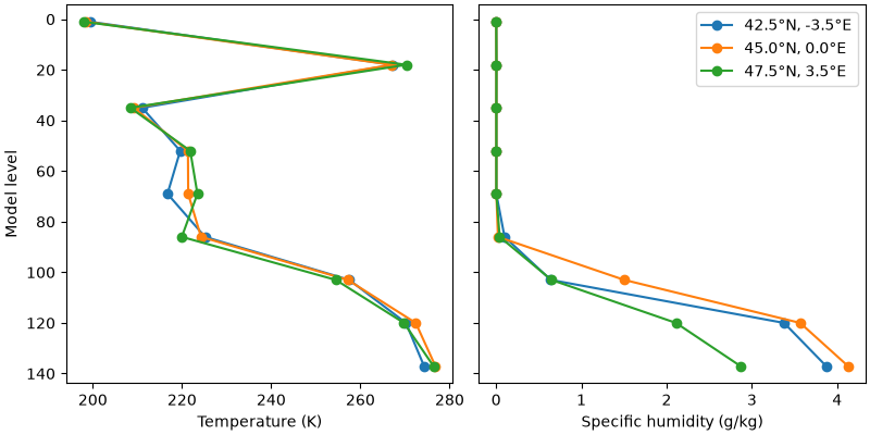
{'t': (3600, 9), 'q': (3600, 9), 'sp': (3600,)}

<matplotlib.legend.Legend object at 0x7d113da93230>

Computing From the Columns

apply() computes values per point from the interpolated columns without holding them all: the columns are interpolated in C++, in parallel, and given to a Python function by blocks of points, with the coordinates of the points and the extra arguments args. Here, the pressure at the altitude of each measurement, reduced from the surface with the virtual temperature of the lowest level, and the dry correction there. The function is an illustration, not the algorithm of a processor.

rng = numpy.random.default_rng(0)
height = rng.uniform(0.0, 500.0, lon.size)
GRAVITY, RD = 9.80665, 287.05


def pressure_at_height(columns, points, a, b):
    """Pressure at the measurement altitude and its dry correction."""
    t, q = columns["t"][:, -1], columns["q"][:, -1]
    virtual = t * (1.0 + 0.608 * q)
    pressure = columns["sp"] * numpy.exp(
        -GRAVITY * points["height"] / (RD * virtual)
    )
    cos2 = numpy.cos(numpy.radians(2.0 * points["lat"]))
    return numpy.stack(
        [pressure, -2.277e-5 * pressure * (1.0 + 0.0026 * cos2)], axis=1
    )


result = rg.apply(
    levels,
    pressure_at_height,
    lon,
    lat,
    dates,
    args={"height": height},
    n_out=2,
)
print(
    f"Pressure at altitude: {result[:, 0].min() / 100:.1f} to "
    f"{result[:, 0].max() / 100:.1f} hPa"
)

Pressure at altitude: 858.6 to 1013.0 hPa

A computation that loops over the levels, such as a vertical integration, does not vectorize over points. column_kernel() compiles it with numba into a native kernel that apply calls for each point, from several threads and without the GIL. The kernel receives the fields concatenated in columns (widths[k] values for field k, in the order of the grid), the hybrid coefficients, and point: the longitude, the latitude, the date (for a series) then the extra arguments. It returns 0, or a non-zero code that makes the point NaN.

if importlib.util.find_spec("numba") is not None:
    import numba

    @rg.column_kernel(n_out=2)
    def kernel(columns, widths, a, b, point, out):
        """Same computation, for one point."""
        n = widths[0]  # t, then q, then sp
        t, q, sp = columns[n - 1], columns[2 * n - 1], columns[2 * n]
        virtual = t * (1.0 + 0.608 * q)
        pressure = sp * numpy.exp(-GRAVITY * point[3] / (RD * virtual))
        cos2 = numpy.cos(numpy.radians(2.0 * point[1]))
        out[0] = pressure
        out[1] = -2.277e-5 * pressure * (1.0 + 0.0026 * cos2)
        return 0

    native = rg.apply(levels, kernel, lon, lat, dates, args={"height": height})
    print(
        f"numba {numba.__version__}: max difference with the Python "
        f"function {numpy.abs(native - result).max():.1e}"
    )
else:
    print("numba is not installed: pip install numba to run the kernel")

numba 0.68.0: max difference with the Python function 0.0e+00

For a series, blend="columns" (the default) blends the columns of the two analyses and calls the function once; blend="results" calls it on the columns of each analysis and blends its results, which costs twice as much: it interpolates in time the result rather than the fields, which differs when the function is nonlinear in them.

by_results = rg.apply(
    levels,
    pressure_at_height,
    lon,
    lat,
    dates,
    args={"height": height},
    n_out=2,
    blend="results",
)
print(
    f"Results minus columns: "
    f"{numpy.abs(by_results - result)[:, 0].max():.2e} Pa"
)

Results minus columns: 1.84e-01 Pa

Reading GRIB Files With ecCodes

pyinterp takes numbers only and never reads GRIB itself. The functions below read a global reduced_gg field with ecCodes (conda install -c conda-forge eccodes python-eccodes) and feed the workflow above. They assume one variable per file and one message per level, as the ECMWF meteorological files of the altimetry processors are delivered.

The mesh and the hybrid coefficients come from the first message:

import os

import eccodes
import numpy as np

from pyinterp import reduced_gaussian as rg


def read_mesh(path):
    """Mesh and hybrid coefficients of the first message of a file."""
    with open(path, "rb") as stream:
        handle = eccodes.codes_grib_new_from_file(stream)
    try:
        if eccodes.codes_get(handle, "gridType") != "reduced_gg":
            raise ValueError("not a reduced Gaussian grid")
        # pyinterp numbers the points from the north, eastwards from 0.
        if (
            eccodes.codes_get(handle, "jScansPositively") != 0
            or eccodes.codes_get(handle, "iScansNegatively") != 0
            or eccodes.codes_get(
                handle, "longitudeOfFirstGridPointInDegrees"
            ) != 0
        ):
            raise ValueError("unsupported scanning mode")
        latitudes = eccodes.codes_get_array(handle, "distinctLatitudes")
        latitudes = np.sort(latitudes)[::-1].copy()  # north to south
        pl = eccodes.codes_get_array(handle, "pl").astype(np.int64)
        a = b = None
        if eccodes.codes_get(handle, "NV") > 0:
            pv = eccodes.codes_get_array(handle, "pv")
            a, b = pv[: len(pv) // 2].copy(), pv[len(pv) // 2 :].copy()
        return rg.Mesh(latitudes, pl), a, b
    finally:
        eccodes.codes_release(handle)


def validity(path):
    """Validity date of the first message of a file."""
    with open(path, "rb") as stream:
        handle = eccodes.codes_grib_new_from_file(stream)
    try:
        date = str(eccodes.codes_get(handle, "validityDate"))
        time = f"{eccodes.codes_get(handle, 'validityTime'):04d}"
        return np.datetime64(
            f"{date[:4]}-{date[4:6]}-{date[6:]}T{time[:2]}:{time[2:]}",
            "ns",
        )
    finally:
        eccodes.codes_release(handle)


def messages(path):
    """Offset of each message of a file, in the order of the levels."""
    offsets = {}
    with open(path, "rb") as stream:
        while (
            handle := eccodes.codes_grib_new_from_file(stream)
        ) is not None:
            try:
                level = eccodes.codes_get(handle, "level")
                offsets[level] = int(eccodes.codes_get(handle, "offset"))
            finally:
                eccodes.codes_release(handle)
    return [offsets[level] for level in sorted(offsets)]

The values of a zone are read in either of two ways. The first decodes each message whole and keeps the points of the zone: it works for any packing, and saves the memory and the copies of the global field:

def read_zone(path, zone):
    """The values of a zone: (points,) or (points, levels)."""
    index = zone.indices()
    columns = []
    with open(path, "rb") as stream:
        for offset in messages(path):
            stream.seek(offset)
            handle = eccodes.codes_grib_new_from_file(stream)
            try:
                columns.append(eccodes.codes_get_values(handle)[index])
            finally:
                eccodes.codes_release(handle)
    return columns[0] if len(columns) == 1 else np.stack(columns, axis=1)

The second reads from the file only the bytes of the zone. It needs the grid_simple packing without bitmap, where value i is an unsigned integer of bitsPerValue bits at a known offset, decoded as \((R + X\,2^E) / 10^D\). On the N640 files of this dataset, reading a regional box this way is five to nine times faster than decoding the messages whole. coalesce merges the ranges closer than io_gap points into one read:

def read_zone_simple(path, zone, io_gap=256):
    """The values of a zone, reading only its bytes (grid_simple)."""
    merged, gather = rg.coalesce(zone.ranges(), io_gap)
    columns = []
    descriptor = os.open(path, os.O_RDONLY)
    try:
        with open(path, "rb") as stream:
            for offset in messages(path):
                stream.seek(offset)
                handle = eccodes.codes_grib_new_from_file(stream)
                try:
                    get = lambda key: eccodes.codes_get(handle, key)
                    if get("packingType") != "grid_simple" or get(
                        "bitmapPresent"
                    ):
                        raise ValueError("use read_zone")
                    size = get("bitsPerValue") // 8
                    if get("bitsPerValue") not in (8, 16, 32):
                        raise ValueError("use read_zone")
                    if get("editionNumber") == 1:
                        first = int(get("offsetSection4")) + 11
                    else:
                        first = int(get("offsetSection7")) + 5
                    reference = get("referenceValue")
                    binary = get("binaryScaleFactor")
                    decimal = get("decimalScaleFactor")
                finally:
                    eccodes.codes_release(handle)
                packed = b"".join(
                    os.pread(
                        descriptor,
                        size * int(stop - start),
                        offset + first + size * int(start),
                    )
                    for start, stop in merged
                )
                raw = np.frombuffer(packed, dtype=f">u{size}")[gather]
                columns.append((reference + raw * 2.0**binary)
                               / 10.0**decimal)
    finally:
        os.close(descriptor)
    return columns[0] if len(columns) == 1 else np.stack(columns, axis=1)

With them, a pass is processed from the files of its analyses, reading for each analysis only the points the pass reads from it:

# One dict per analysis: field name -> GRIB file.
files = {
    validity(paths["t"]): paths
    for paths in (
        {"t": "T3A_12h.grib", "q": "Q3A_12h.grib", "sp": "PRA_12h.grib"},
        {"t": "T3A_18h.grib", "q": "Q3A_18h.grib", "sp": "PRA_18h.grib"},
    )
}
steps = np.array(sorted(files))
mesh, a, b = read_mesh(files[steps[0]]["t"])
interval = np.timedelta64(6, "h")

# lon, lat, dates: the measurements of the pass.
zones = rg.time_zones(mesh, steps, dates, lon, lat, interval=interval)
series = rg.Series(mesh)
for step, zone in zip(steps, zones):
    if zone.size == 0:  # no measurement reads this analysis
        continue
    fields = {
        name: read_zone_simple(path, zone)
        for name, path in files[step].items()
    }
    series.append(step, rg.Grid(mesh, fields, zone=zone, a=a, b=b))

columns = rg.interpolate(series, lon, lat, dates, interval=interval)
flags = rg.map_availability(steps, dates, interval)

The 3D fields come back with the levels in the order of the GRIB level key, top of the atmosphere first, as the coefficients a and b.