Conservative Regridding

Interpolating a fine grid onto a coarse one samples it: each target value comes from the few source nodes around a point, and the small scales between the target points are lost or aliased. Conservative regridding averages it instead: each target cell receives the mean of the source values weighted by the area of their overlap with the cell, which preserves the integral of the field. In this example you will learn how to coarsen a grid with the pyinterp accessor, handle undefined values, regrid a variable with a time dimension, and average over a single box.

import matplotlib.pyplot
import numpy

import pyinterp
import pyinterp.backends.xarray
import pyinterp.tests

Coarsening a Grid

We load the global mean sea surface (MSS) at 0.25°, stored as (lat, lon) with longitudes in [0, 360) and NaN over land. The regrid() method takes the centers of the target cells as keyword arguments, like interp(): here a 2° grid in [-180, 180). The longitude and latitude are recognized from their units, and the bounds of the cells are the midpoints between the centers.

mss = pyinterp.tests.load_grid2d().mss
lon = numpy.arange(-180, 180, 2.0) + 1
lat = numpy.arange(-90, 90, 2.0) + 1
conservative = mss.pyinterp.regrid(lon=lon, lat=lat)
bilinear = mss.pyinterp.interp(lon=lon, lat=lat)
print(conservative)

<xarray.DataArray 'mss' (lat: 90, lon: 180)> Size: 130kB
array([[nan, nan, nan, ..., nan, nan, nan],
       [nan, nan, nan, ..., nan, nan, nan],
       [nan, nan, nan, ..., nan, nan, nan],
       ...,
       [nan, nan, nan, ..., nan, nan, nan],
       [nan, nan, nan, ..., nan, nan, nan],
       [nan, nan, nan, ..., nan, nan, nan]], shape=(90, 180))
Coordinates:
  * lat      (lat) float64 720B -89.0 -87.0 -85.0 -83.0 ... 83.0 85.0 87.0 89.0
  * lon      (lon) float64 1kB -179.0 -177.0 -175.0 -173.0 ... 175.0 177.0 179.0
Attributes:
    long_name:     Mean sea surface height above reference ellipsoid
    units:         m
    grid_mapping:  crs
    source:        SMO15_1s60_V2.dat
    cell_methods:  lon: point lat: point

The undefined values are ignored: a coastal cell gets the mean of its ocean part, so the conservative regridding keeps cells that the bilinear interpolation loses as soon as one of the four surrounding nodes is on land.

print(
    f"Defined cells: conservative={int(conservative.notnull().sum())}, "
    f"bilinear={int(bilinear.notnull().sum())}"
)
fig, (ax1, ax2) = matplotlib.pyplot.subplots(
    2, 1, figsize=(10, 7), sharex=True, layout="constrained"
)
pcm = ax1.pcolormesh(lon, lat, conservative, vmin=-0.1, vmax=0.1)
fig.colorbar(pcm, ax=ax1, label="MSS (m)")
ax1.set_title("Conservative regridding onto 2° cells")
pcm = ax2.pcolormesh(
    lon,
    lat,
    (conservative - bilinear) * 1e3,
    cmap="RdBu_r",
    vmin=-2,
    vmax=2,
)
fig.colorbar(pcm, ax=ax2, label="mm")
ax2.set_title("Conservative minus bilinear")
ax2.set_xlabel("Longitude (degrees)")
for ax in (ax1, ax2):
    ax.set_ylabel("Latitude (degrees)")

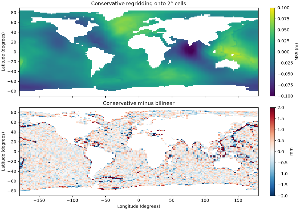
Defined cells: conservative=11099, bilinear=9752

Preserving the Integral

The area of a longitude/latitude cell is proportional to its width in longitude times the difference of the sines of its latitudes, which pyinterp.regrid.cell_bounds() gives from the centers of the cells. With normalize=False, the undefined values count as zero: the integral of the field over the sphere is then preserved exactly.

def integral(data, lon_name="lon", lat_name="lat"):
    """Integral of a field over the sphere of radius 1, NaN counting as 0."""
    x = pyinterp.regrid.cell_bounds(data[lon_name].values, "longitude")
    y = pyinterp.regrid.cell_bounds(data[lat_name].values, "latitude")
    areas = numpy.outer(
        numpy.diff(numpy.sin(numpy.radians(y)))[:, 0],
        numpy.radians(numpy.diff(x)[:, 0]),
    )
    return numpy.nansum(data.values * areas)


zero = mss.pyinterp.regrid(lon=lon, lat=lat, normalize=False)
print(f"Integral on the 0.25° grid: {integral(mss):.10f}")
print(f"Integral on the 2° grid:    {integral(zero):.10f}")

Integral on the 0.25° grid: 0.0076671459
Integral on the 2° grid:    0.0076671459

With min_valid_fraction, a cell whose defined values cover less than this fraction of its area is undefined: with 1, only the cells entirely over the ocean keep a value.

ocean_only = mss.pyinterp.regrid(lon=lon, lat=lat, min_valid_fraction=1.0)
print(f"Cells entirely over the ocean: {int(ocean_only.notnull().sum())}")

Cells entirely over the ocean: 6729

Other Dimensions

The dimensions that are not regridded, such as the time, are kept with their coordinates. Here the daily total column water vapor, stored as (time, latitude, longitude), is coarsened to 2.5° in one call.

tcw = pyinterp.tests.load_grid3d().tcw
daily = tcw.pyinterp.regrid(
    longitude=numpy.arange(0, 360, 2.5) + 1.25,
    latitude=numpy.arange(-80, 80, 2.5) + 1.25,
)
print(daily.dims, daily.shape)

('time', 'latitude', 'longitude') (31, 64, 144)

Averaging over a Box

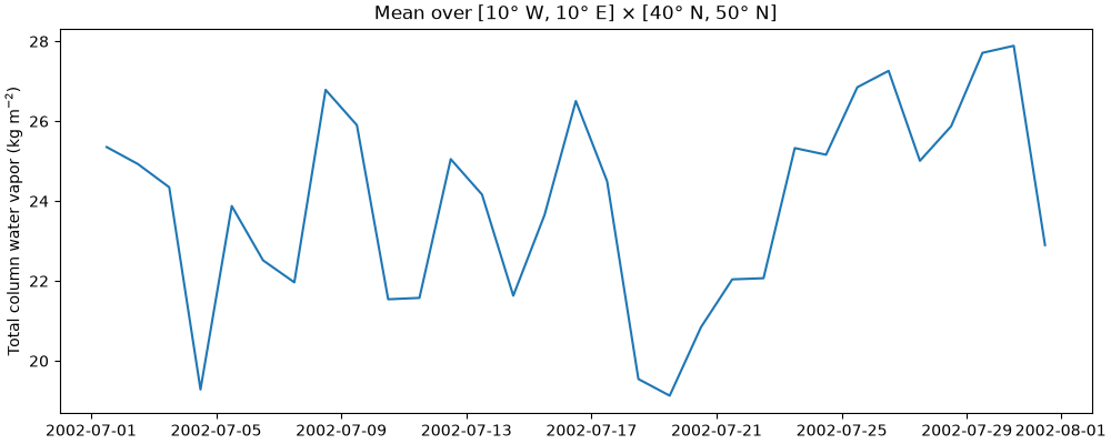
A dimension of a single cell cannot be inferred from its center: give the bounds of the cells instead, an array of shape (n, 2). The mean water vapor over the box [10° W, 10° E] × [40° N, 50° N] is a time series.

box = tcw.pyinterp.regrid(
    longitude=[[-10.0, 10.0]], latitude=[[40.0, 50.0]]
).squeeze()
fig, ax = matplotlib.pyplot.subplots(figsize=(10, 4), layout="constrained")
ax.plot(box.time, box)
ax.set_ylabel("Total column water vapor (kg m$^{-2}$)")
ax.set_title("Mean over [10° W, 10° E] × [40° N, 50° N]")

Text(0.5, 1.0, 'Mean over [10° W, 10° E] × [40° N, 50° N]')