Tide Prediction from Known Constituents

This example shows how to use evaluate_tide_from_constituents to predict tides when you already know the tidal constituents at a location.

This example uses real harmonic analysis results from the Brest tide gauge (France), obtained from the TICON-3 database. The data represents constituents derived from over 100 years of observations (1846-2021).

Reference: Hart-Davis, Michael G; Dettmering, Denise; Seitz, Florian (2022). TICON-3: Tidal Constants based on GESLA-3 sea-level records from globally distributed tide gauges including gauge type information (data) [dataset]. PANGAEA. https://doi.org/10.1594/PANGAEA.951610

from __future__ import annotations

import matplotlib.pyplot as plt
import numpy as np
import pyfes

Load Real Tide Gauge Constituents from TICON-3

These constituents are from the Brest tide gauge (48.383°N, 4.495°W), one of the oldest and most reliable tide gauges in the world.

Complete TICON-3 data for Brest (gesla.uhslc dataset)

BREST_TICON3_DATA = {
    'M2': (205.113, 109.006),
    'K1': (6.434, 75.067),
    'N2': (41.695, 90.633),
    'O1': (6.587, 327.857),
    'P1': (2.252, 63.658),
    'Q1': (2.040, 281.362),
    'K2': (21.361, 145.892),
    'S2': (74.876, 148.283),
    'S1': (0.797, 11.441),
    'SA': (4.905, 322.761),
    'T2': (4.171, 138.535),
    'MF': (1.031, 175.663),
    'MM': (0.425, 199.741),
    '2N2': (5.699, 72.786),
    'M4': (5.437, 105.940),
    'J1': (0.241, 123.005),
    'SSA': (2.047, 98.898),
    'MSF': (0.356, 24.980),
    'MSQM': (0.115, 254.934),  # Noted as MSQ in TICON-3
    'EPS2': (1.968, 89.471),  # Noted as EP2 in TICON-3
    'L2': (6.392, 102.910),
    'M3': (1.977, 15.860),
    'R2': (0.534, 158.066),
    'MU2': (8.566, 105.087),  # Noted as MI2 in TICON-3
    'MTM': (0.110, 142.031),
    'NU2': (7.780, 86.614),  # Noted as NI2 in TICON-3
    'LAMBDA2': (2.625, 75.845),  # Noted as LM2 in TICON-3
    'MN4': (1.937, 60.491),
    'MS4': (3.258, 181.835),
    'MKS2': (0.758, 173.969),  # Noted as MKS in TICON-3
    'N4': (0.291, 9.263),
    'M6': (3.153, 354.764),
    'M8': (0.231, 231.883),
    'S4': (0.217, 289.151),
    '2Q1': (0.376, 234.893),
    'OO1': (0.136, 213.353),
    'S3': (0.308, 149.130),
    'MA2': (1.106, 39.588),
    'MB2': (1.252, 101.029),
    'M1': (0.535, 83.038),
}
BREST_LON = -4.495  # degrees East
BREST_LAT = 48.383  # degrees North

Parse and Filter Constituents

We’ll attempt to parse each constituent name and filter to only those recognized by pyfes. This is the realistic workflow when working with external harmonic analysis results.

constituents = {}
skipped = []

print(
    f'\n{"Constituent":<12} {"Amplitude (cm)":<16} '
    f'{"Phase (deg)":<14} {"Status"}'
)
print('-' * 70)

for name, (amplitude, phase) in BREST_TICON3_DATA.items():
    try:
        # Try to parse the constituent name - this will raise if unknown
        constituent_id = pyfes.constituents.parse(name)
        constituents[constituent_id] = (amplitude, phase)
        print(f'{name:<12} {amplitude:>15.3f} {phase:>13.3f}  ✓ included')
    except ValueError:
        # Constituent not recognized by pyfes
        skipped.append((name, amplitude, phase))
        print(f'{name:<12} {amplitude:>15.3f} {phase:>13.3f}  ✗ not in pyfes')

print('-' * 70)
print(f'Constituents included: {len(constituents)}')
print(f'Constituents skipped: {len(skipped)}')
print('=' * 70)

if skipped:
    print('\nSkipped constituents (not recognized by pyfes):')
    total_skipped_amplitude = sum(amp for _, amp, _ in skipped)
    for name, amp, phase in sorted(skipped, key=lambda x: x[1], reverse=True):
        print(f'  {name:<12} amplitude: {amp:6.3f} cm, phase: {phase:6.3f}°')

Constituent  Amplitude (cm)   Phase (deg)    Status
----------------------------------------------------------------------
M2                   205.113       109.006  ✓ included
K1                     6.434        75.067  ✓ included
N2                    41.695        90.633  ✓ included
O1                     6.587       327.857  ✓ included
P1                     2.252        63.658  ✓ included
Q1                     2.040       281.362  ✓ included
K2                    21.361       145.892  ✓ included
S2                    74.876       148.283  ✓ included
S1                     0.797        11.441  ✓ included
SA                     4.905       322.761  ✓ included
T2                     4.171       138.535  ✓ included
MF                     1.031       175.663  ✓ included
MM                     0.425       199.741  ✓ included
2N2                    5.699        72.786  ✓ included
M4                     5.437       105.940  ✓ included
J1                     0.241       123.005  ✓ included
SSA                    2.047        98.898  ✓ included
MSF                    0.356        24.980  ✓ included
MSQM                   0.115       254.934  ✓ included
EPS2                   1.968        89.471  ✓ included
L2                     6.392       102.910  ✓ included
M3                     1.977        15.860  ✓ included
R2                     0.534       158.066  ✓ included
MU2                    8.566       105.087  ✓ included
MTM                    0.110       142.031  ✓ included
NU2                    7.780        86.614  ✓ included
LAMBDA2                2.625        75.845  ✓ included
MN4                    1.937        60.491  ✓ included
MS4                    3.258       181.835  ✓ included
MKS2                   0.758       173.969  ✓ included
N4                     0.291         9.263  ✓ included
M6                     3.153       354.764  ✓ included
M8                     0.231       231.883  ✓ included
S4                     0.217       289.151  ✓ included
2Q1                    0.376       234.893  ✓ included
OO1                    0.136       213.353  ✓ included
S3                     0.308       149.130  ✗ not in pyfes
MA2                    1.106        39.588  ✗ not in pyfes
MB2                    1.252       101.029  ✗ not in pyfes
M1                     0.535        83.038  ✓ included
----------------------------------------------------------------------
Constituents included: 37
Constituents skipped: 3
======================================================================

Skipped constituents (not recognized by pyfes):
  MB2          amplitude:  1.252 cm, phase: 101.029°
  MA2          amplitude:  1.106 cm, phase: 39.588°
  S3           amplitude:  0.308 cm, phase: 149.130°

Set Up Prediction Parameters

Define the time period for tide prediction at Brest.

# Time period: 30 days with 10-minute resolution
start_date = np.datetime64('2025-06-01T00:00:00')
end_date = np.datetime64('2025-07-01T00:00:00')
dates = np.arange(start_date, end_date, np.timedelta64(10, 'm'))
print(f"""Prediction Settings:
    Location: Brest, France
    Coordinates: {BREST_LAT:.3f}°N, {BREST_LON:.3f}°W
    Period: {start_date} to {end_date}
    Time points: {len(dates)} (10-minute intervals)
""")

Prediction Settings:
    Location: Brest, France
    Coordinates: 48.383°N, -4.495°W
    Period: 2025-06-01T00:00:00 to 2025-07-01T00:00:00
    Time points: 4320 (10-minute intervals)

Predict Tides

Call evaluate_tide_from_constituents() to compute the tide at Brest using the observed tidal constituents.

tide, long_period = pyfes.evaluate_tide_from_constituents(
    constituents,
    dates,
    BREST_LON,
    BREST_LAT,
)

# Total sea level from tides
total_tide = tide + long_period
print(f"""Prediction Results:
    Short-period tide range: {tide.min():.1f} - {tide.max():.1f} cm
    Long-period tide range: {long_period.min():.1f} - {long_period.max():.1f} cm
    Total tide range: {total_tide.min():.1f} - {total_tide.max():.1f} cm
    Tidal amplitude: {(total_tide.max() - total_tide.min()) / 2:.1f} cm
""")

Prediction Results:
    Short-period tide range: -291.7 - 285.2 cm
    Long-period tide range: -4.9 - 1.3 cm
    Total tide range: -293.6 - 283.4 cm
    Tidal amplitude: 288.5 cm

Find High and Low Tides

Identify the times and heights of high and low tides.

def find_extrema(times, values):
    """Find local maxima and minima."""
    maxima_idx = []
    minima_idx = []

    for i in range(1, len(values) - 1):
        if values[i] > values[i - 1] and values[i] > values[i + 1]:
            maxima_idx.append(i)
        elif values[i] < values[i - 1] and values[i] < values[i + 1]:
            minima_idx.append(i)

    return (
        times[maxima_idx],
        values[maxima_idx],
        times[minima_idx],
        values[minima_idx],
    )


high_times, high_values, low_times, low_values = find_extrema(dates, total_tide)

print(f"""Tidal Statistics (30 days):
      Number of high tides: {len(high_times)}
      Number of low tides: {len(low_times)}
      Average high tide: {high_values.mean():.1f} cm
      Average low tide: {low_values.mean():.1f} cm
""")

# Show first few high and low tides
print('\nFirst 5 High Tides:')
for i in range(min(5, len(high_times))):
    print(f'  {high_times[i]}: {high_values[i]:.1f} cm')

print('\nFirst 5 Low Tides:')
for i in range(min(5, len(low_times))):
    print(f'  {low_times[i]}: {low_values[i]:.1f} cm')

Tidal Statistics (30 days):
      Number of high tides: 58
      Number of low tides: 58
      Average high tide: 201.0 cm
      Average low tide: -208.4 cm


First 5 High Tides:
  2025-06-01T07:50:00: 176.5 cm
  2025-06-01T20:10:00: 190.6 cm
  2025-06-02T08:40:00: 148.3 cm
  2025-06-02T21:10:00: 162.6 cm
  2025-06-03T09:50:00: 130.9 cm

First 5 Low Tides:
  2025-06-01T01:50:00: -219.2 cm
  2025-06-01T14:10:00: -184.1 cm
  2025-06-02T02:40:00: -188.0 cm
  2025-06-02T15:00:00: -158.9 cm
  2025-06-03T03:40:00: -163.6 cm

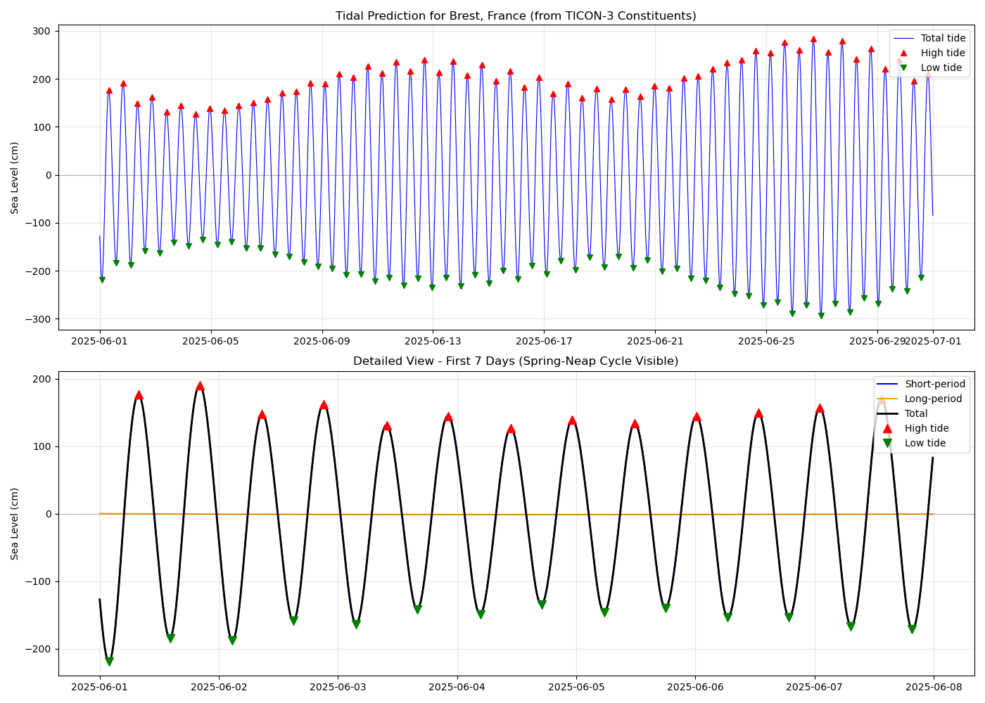
Visualize the Results

Create plots showing the predicted tide over different time scales.

fig, axes = plt.subplots(2, 1, figsize=(14, 10))

# Plot 1: Full 30-day period
ax = axes[0]
ax.plot(dates, total_tide, 'b-', linewidth=0.8, label='Total tide')
ax.plot(high_times, high_values, 'r^', markersize=6, label='High tide')
ax.plot(low_times, low_values, 'gv', markersize=6, label='Low tide')
ax.axhline(y=0, color='k', linestyle='--', linewidth=0.5, alpha=0.5)
ax.set_ylabel('Sea Level (cm)')
ax.set_title('Tidal Prediction for Brest, France (from TICON-3 Constituents)')
ax.grid(True, alpha=0.3)
ax.legend(loc='upper right')

# Plot 2: Detailed view of first 7 days
ax = axes[1]
days_7 = 7 * 24 * 6  # 7 days at 10-minute intervals
ax.plot(
    dates[:days_7], tide[:days_7], 'b-', linewidth=1.5, label='Short-period'
)
ax.plot(
    dates[:days_7],
    long_period[:days_7],
    'orange',
    linewidth=1.5,
    label='Long-period',
)
ax.plot(dates[:days_7], total_tide[:days_7], 'k-', linewidth=2, label='Total')

# Mark high and low tides in this period
mask_7days = high_times < dates[days_7]
ax.plot(
    high_times[mask_7days],
    high_values[mask_7days],
    'r^',
    markersize=8,
    label='High tide',
)
mask_7days = low_times < dates[days_7]
ax.plot(
    low_times[mask_7days],
    low_values[mask_7days],
    'gv',
    markersize=8,
    label='Low tide',
)

ax.axhline(y=0, color='k', linestyle='--', linewidth=0.5, alpha=0.5)
ax.set_ylabel('Sea Level (cm)')
ax.set_title('Detailed View - First 7 Days (Spring-Neap Cycle Visible)')
ax.grid(True, alpha=0.3)
ax.legend(loc='upper right')

plt.tight_layout()
plt.show()