Prediction example

In this example, we will use the model to predict the tidal elevation on a specific location, like a tide gauge.

Warning

The model employed is an older FES tidal-atlas model due to its significantly smaller size compared to newer models. Do not use it for real applications. You can download the model from the AVISO website.

First, we import the required modules.

from __future__ import annotations

import os
import pathlib

from IPython.display import HTML
import markdown
import matplotlib.pyplot as plt
import numpy

import pyfes

To display properly formatted markdown tables in this notebook, we define a helper function that converts markdown strings to HTML.

def md_to_html(md_string: str) -> HTML:
    """Convert a markdown string to HTML for display in Jupyter."""
    html_string = markdown.markdown(md_string, extensions=['tables'])
    return HTML(html_string)

Loading the model configuration

First we create an environment variable to store the path to the model file.

os.environ['DATASET_DIR'] = str(
    pathlib.Path().absolute().parent / 'tests' / 'python' / 'dataset'
)

Now we need to create the instances of the model used to calculate the ocean tide and the radial tide. To do this, we need to create a YAML file that describes the models and their parameters. The configuration file is fully documented in the documentation.

Note

The content of the configuration file is viewable in the GitHub repository.

config = pyfes.config.load(pathlib.Path().absolute() / 'fes_slev.yml')

Hint

By default, the function pyfes.config.load() loads the entire numeric grid into memory. To predict the tide for a specific region, you can use the bbox keyword argument to specify the region’s bounding box. This bounding box is a tuple of four elements: minimum longitude, minimum latitude, maximum longitude, and maximum latitude. Example:

config = pyfes.config.load('fes_slev.yaml', bbox=(-10, 40, 10, 60))

config is a Configuration namedtuple that contains the tidal models and the runtime settings loaded from the configuration file.

print(config)

Configuration(models={'radial': TidalModelInterface(9 constituents, tide_type=RADIAL), 'tide': TidalModelInterface(15 constituents, tide_type=TIDE)}, settings=<FESSettings num_threads=0>)

Prediction Engine Information

This configuration uses the FES/Darwin engine, which employs Darwin’s harmonic notation with Schureman’s nodal corrections. This is the classical engine designed for FES tidal atlases.

The Darwin engine:

• Uses fundamental astronomical arguments (s, h, p, N, p₁)

• Applies individual Schureman nodal corrections to each constituent

• Supports 99 tidal constituents

• Uses traditional admittance for minor constituents

To use the PERTH/Doodson engine instead (for GOT tidal models), set engine: perth in your YAML configuration. The PERTH engine uses Doodson number classification and group modulations. See the engine comparison example for details on choosing between engines.

print(f'\nRuntime Settings: {type(config.settings).__name__}')
print('Engine: FES/Darwin (Schureman nodal corrections)')
print(f'Astronomical formulae: {config.settings.astronomic_formulae}')
print(f'Time tolerance: {config.settings.time_tolerance} seconds')

Runtime Settings: FESSettings
Engine: FES/Darwin (Schureman nodal corrections)
Astronomical formulae: Formulae.SCHUREMAN_ORDER_1
Time tolerance: 0.0 seconds

Displaying the Configuration as a Markdown Table

You can generate a markdown table summarizing the engine settings and the constituent list (modeled vs. inferred) using pyfes.generate_markdown_table(). Pass the settings and the list of modeled constituents to see which ones are provided by the atlas and which ones will be inferred.

md_to_html(
    pyfes.generate_markdown_table(
        config.settings,
        modeled_constituents=config.models['tide'].identifiers(),
    )
)

Setting	Value
Engine Type	Darwin
Astronomic Formulae	Schureman Order 1
Inference Type	Spline
Time Tolerance (s)	0.000000
Group Modulations	N/A
Compute Long Period Equilibrium	Yes
Number of Threads	0

Constituent	Speed (Deg/hr)	XDO	Modeled	Inferred
Mm	0.544375	ZAZYZZZ	Yes	No
Mf	1.098033	ZBZZZZZ	Yes	No
Mtm	1.642408	ZCZYZZZ	Yes	No
MSqm	2.113929	ZDXZZZZ	Yes	No
2Q1	12.854286	AWZBZZY	No	Yes
${\sigma}1$	12.927140	AWBZZZY	No	Yes
Q1	13.398661	AXZAZZY	Yes	No
${\rho}1$	13.471515	AXBYZZY	No	Yes
O1	13.943036	AYZZZZY	Yes	No
M11	14.487410	AZZYZZA	No	Yes
M12	14.496694	AZZAZZA	No	Yes
${\chi}1$	14.569548	AZBYZZA	No	Yes
${\pi}1$	14.917865	AAWZZAY	No	Yes
P1	14.958931	AAXZZZY	Yes	No
S1	15.000000	AAYZZZZ	Yes	No
K1	15.041069	AAZZZZA	Yes	No
${\phi}1$	15.123206	AABZZZA	No	Yes
${\theta}1$	15.512590	ABXAZZA	No	Yes
J1	15.585443	ABZYZZA	No	Yes
OO1	16.139102	ACZZZZA	No	Yes
${\epsilon}2$	27.423834	BWBAZZZ	No	Yes
2N2	27.895355	BXZBZZZ	Yes	No
${\mu}2$	27.968208	BXBZZZZ	No	Yes
N2	28.439730	BYZAZZZ	Yes	No
${\nu}2$	28.512583	BYBYZZZ	No	Yes
M2	28.984104	BZZZZZZ	Yes	No
${\lambda}2$	29.455625	BAXAZZB	No	Yes
L2	29.528479	BAZYZZB	No	Yes
T2	29.958933	BBWZZAZ	No	Yes
S2	30.000000	BBXZZZZ	Yes	No
K2	30.082137	BBZZZZZ	Yes	No
${\eta}2$	30.626512	BCZYZZZ	No	Yes
M4	57.968208	DZZZZZZ	Yes	No

Generating the tide prediction

Set up the position and the dates where we want to calculate the tide.

lon = -7.688
lat = 59.195
date = numpy.datetime64('1983-01-01T00:00:00')

Generate the coordinates where we want to calculate the tide.

dates = numpy.arange(
    date, date + numpy.timedelta64(1, 'D'), numpy.timedelta64(1, 'h')
)
lons = numpy.full(dates.shape, lon)
lats = numpy.full(dates.shape, lat)

We can now calculate the ocean tide and the radial tide.

tide, lp, _ = pyfes.evaluate_tide(
    config.models['tide'], dates, lons, lats, settings=config.settings
)
load, load_lp, _ = pyfes.evaluate_tide(
    config.models['radial'], dates, lons, lats, settings=config.settings
)

Displaying the results

Calculate CNES Julian Days (days since 1950-01-01). This is the standard time reference used in CNES altimetry products.

cnes_julian_days = (dates - numpy.datetime64('1950-01-01T00:00:00')).astype(
    'M8[s]'
).astype(float) / 86400
hours = cnes_julian_days % 1 * 24
print(
    f'{"JulDay":>6s} {"Hour":>5s} {"Latitude":>10s} {"Longitude":>10s} '
    f'{"Short_tide":>10s} {"LP_tide":>10s} {"Pure_Tide":>10s} '
    f'{"Geo_Tide":>10s} {"Rad_Tide":>10s}'
)
print('=' * 89)
for ix, jd in enumerate(cnes_julian_days):
    print(
        f'{jd:>6.0f} {hours[ix]:>5.0f} {lats[ix]:>10.3f} {lons[ix]:>10.3f} '
        f'{tide[ix]:>10.3f} {lp[ix]:>10.3f} {tide[ix] + lp[ix]:>10.3f} '
        f'{tide[ix] + lp[ix] + load[ix]:>10.3f} {load[ix]:>10.3f}'
    )

JulDay  Hour   Latitude  Longitude Short_tide    LP_tide  Pure_Tide   Geo_Tide   Rad_Tide
=========================================================================================
 12053     0     59.195     -7.688   -100.991      0.896   -100.095    -96.214      3.881
 12053     1     59.195     -7.688   -137.105      0.869   -136.236   -131.907      4.328
 12053     2     59.195     -7.688   -138.483      0.842   -137.641   -133.930      3.711
 12053     3     59.195     -7.688   -104.346      0.814   -103.532   -101.398      2.134
 12053     4     59.195     -7.688    -42.516      0.785    -41.731    -41.783     -0.052
 12053     5     59.195     -7.688     32.374      0.756     33.130     30.789     -2.341
 12053     6     59.195     -7.688    102.167      0.726    102.893     98.699     -4.194
 12053     7     59.195     -7.688    149.469      0.696    150.165    144.993     -5.172
 12053     8     59.195     -7.688    162.102      0.665    162.767    157.722     -5.046
 12053     9     59.195     -7.688    136.505      0.634    137.139    133.287     -3.852
 12053    10     59.195     -7.688     78.896      0.602     79.498     77.613     -1.885
 12053    11     59.195     -7.688      3.645      0.570      4.215      4.597      0.382
 12054    12     59.195     -7.688    -70.659      0.537    -70.121    -67.711      2.411
 12054    13     59.195     -7.688   -126.152      0.504   -125.647   -121.914      3.734
 12054    14     59.195     -7.688   -150.115      0.471   -149.644   -145.573      4.071
 12054    15     59.195     -7.688   -137.779      0.437   -137.342   -133.949      3.393
 12054    16     59.195     -7.688    -93.132      0.403    -92.729    -90.801      1.928
 12054    17     59.195     -7.688    -27.820      0.369    -27.451    -27.354      0.097
 12054    18     59.195     -7.688     41.541      0.334     41.875     40.282     -1.593
 12054    19     59.195     -7.688     97.250      0.299     97.549     94.865     -2.684
 12054    20     59.195     -7.688    124.939      0.263    125.203    122.321     -2.882
 12054    21     59.195     -7.688    117.465      0.228    117.693    115.561     -2.132
 12054    22     59.195     -7.688     77.026      0.192     77.218     76.583     -0.635
 12054    23     59.195     -7.688     14.661      0.156     14.817     16.027      1.210

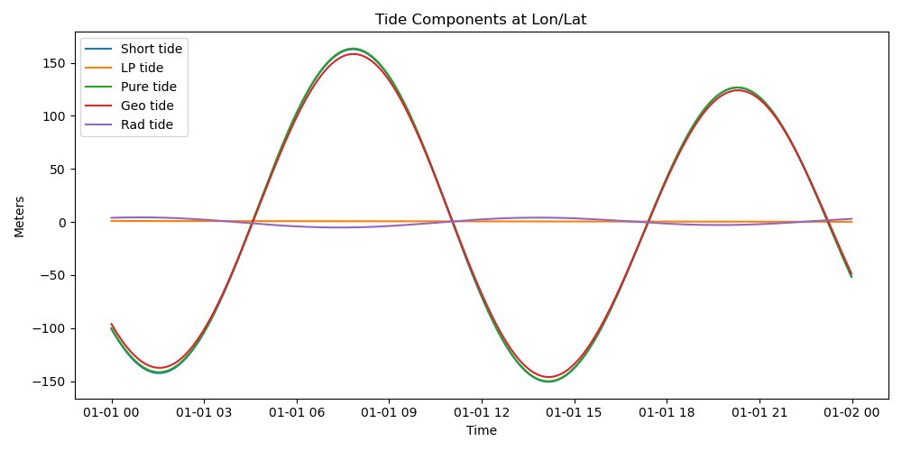
Plot the tide components shown in the table. We recompute the tide only to generate smoother curves on the figure below.

dates = numpy.arange(
    date, date + numpy.timedelta64(1, 'D'), numpy.timedelta64(1, 'm')
)
lons = numpy.full(dates.shape, lon)
lats = numpy.full(dates.shape, lat)
tide, lp, _ = pyfes.evaluate_tide(
    config.models['tide'], dates, lons, lats, settings=config.settings
)
load, load_lp, _ = pyfes.evaluate_tide(
    config.models['radial'], dates, lons, lats, settings=config.settings
)

pure_tide = tide + lp
geo_tide = pure_tide + load

plt.figure(figsize=(10, 5))
plt.plot(dates, tide, label='Short tide')
plt.plot(dates, lp, label='LP tide')
plt.plot(dates, pure_tide, label='Pure tide')
plt.plot(dates, geo_tide, label='Geo tide')
plt.plot(dates, load, label='Rad tide')
plt.title('Tide Components at Lon/Lat')
plt.xlabel('Time')
plt.ylabel('Meters')
plt.legend()
plt.tight_layout()