Harmonic Analysis

This example demonstrates how to perform harmonic analysis on a signal using the harmonic_analysis method.

First, we import the required modules.

from __future__ import annotations

import pathlib

import matplotlib.pyplot
import netCDF4

import pyfes

The distribution contains a time series fes_tide_time_series.nc that will be used in this example.

SIGNAL = (
    pathlib.Path().absolute().parent
    / 'tests'
    / 'python'
    / 'dataset'
    / 'fes_tide_time_series.nc'
)

Load the signal.

with netCDF4.Dataset(SIGNAL, 'r') as ds:
    time = (ds.variables['time'][:]).astype('datetime64[us]')
    h = ds['ocean'][:] * 1e-2  # cm to m

Then, we will create an instance of a pyfes.WaveTableInterface object. This class handles and retrieves the properties of the tidal waves supported by the prediction engine.

wt = pyfes.wave_table_factory(pyfes.DARWIN)

By default, all tidal components are loaded into memory. Use pyfes.known_constituents() to retrieve the list of available tidal constituents in pyfes.

print(pyfes.known_constituents())

['2MK2', '2MK3', '2MK6', '2MN2', '2MN6', '2MNS4', '2MP5', '2MS2', '2MS6', '2MSN4', '2N2', '2NM6', '2NS2', '2Q1', '2SM2', '2SM6', '2SMu2', '3MS4', '3MS8', 'A5', 'Alpha2', 'Beta1', 'Beta2', 'Chi1', 'Delta2', 'Eps2', 'Eta2', 'Gamma2', 'J1', 'K1', 'K2', 'L2', 'L2P', 'Lambda2', 'M0', 'M1', 'M11', 'M12', 'M13', 'M2', 'M3', 'M4', 'M6', 'M8', 'Mf', 'Mf1', 'Mf2', 'MK3', 'MK4', 'MKS2', 'ML4', 'Mm', 'Mm1', 'Mm2', 'MN4', 'MNK6', 'MNS2', 'MNu4', 'MNuS2', 'MO3', 'MP1', 'Mqm', 'MS4', 'MSf', 'MSK2', 'MSK6', 'MSm', 'MSN2', 'MSN6', 'MSqm', 'MStm', 'Mtm', 'Mu2', 'N2', 'N2P', 'N4', 'NK4', 'NKM2', 'Node', 'Nu2', 'O1', 'OO1', 'OQ2', 'P1', 'Phi1', 'Pi1', 'Psi1', 'Q1', 'R2', 'R4', 'Rho1', 'S1', 'S2', 'S4', 'S6', 'Sa', 'Sa1', 'Sigma1', 'SK3', 'SK4', 'SKM2', 'SN4', 'SO1', 'SO3', 'Ssa', 'Sta', 'T2', 'Tau1', 'Theta1', 'Ups1']

If you want to restrict the analysis to only a few components, either pass a list of waves to the constructor or call select_waves_for_analysis() to automatically choose them based on the time-series length.

See also

The Rayleigh Criterion for the physical explanation of how the Rayleigh Criterion separates tidal constituents.

In this example, we overwrite the previous WaveTable with a new one that includes a specific list of constituents tailored for this dataset. This ensures the analysis focuses on the relevant tidal components present in the signal.

wt = pyfes.wave_table_factory(
    pyfes.DARWIN,
    [
        'Mm',
        'Mf',
        'Mtm',
        'Msqm',
        '2Q1',
        'Sigma1',
        'Q1',
        'Rho1',
        'O1',
        'MP1',
        'M11',
        'M12',
        'M13',
        'Chi1',
        'Pi1',
        'P1',
        'S1',
        'K1',
        'Psi1',
        'Phi1',
        'Theta1',
        'J1',
        'OO1',
        'MNS2',
        'Eps2',
        '2N2',
        'Mu2',
        '2MS2',
        'N2',
        'Nu2',
        'M2',
        'MKS2',
        'Lambda2',
        'L2',
        '2MN2',
        'T2',
        'S2',
        'R2',
        'K2',
        'MSN2',
        'Eta2',
        '2SM2',
        'MO3',
        '2MK3',
        'M3',
        'MK3',
        'N4',
        'MN4',
        'M4',
        'SN4',
        'MS4',
        'MK4',
        'S4',
        'SK4',
        'R4',
        '2MN6',
        'M6',
        'MSN6',
        '2MS6',
        '2MK6',
        '2SM6',
        'MSK6',
        'S6',
        'M8',
        'MSf',
        'Ssa',
        'Sa',
    ],
)

The constituents property returns the list of tidal constituent names supported by this wave table instance:

print(wt.constituents)

['2MK3', '2MK6', '2MN2', '2MN6', '2MS2', '2MS6', '2N2', '2Q1', '2SM2', '2SM6', 'Chi1', 'Eps2', 'Eta2', 'J1', 'K1', 'K2', 'L2', 'Lambda2', 'M11', 'M12', 'M13', 'M2', 'M3', 'M4', 'M6', 'M8', 'Mf', 'MK3', 'MK4', 'MKS2', 'Mm', 'MN4', 'MNS2', 'MO3', 'MP1', 'MS4', 'MSf', 'MSK6', 'MSN2', 'MSN6', 'MSqm', 'Mtm', 'Mu2', 'N2', 'N4', 'Nu2', 'O1', 'OO1', 'P1', 'Phi1', 'Pi1', 'Psi1', 'Q1', 'R2', 'R4', 'Rho1', 'S1', 'S2', 'S4', 'S6', 'Sa', 'Sigma1', 'SK4', 'SN4', 'Ssa', 'T2', 'Theta1']

The different nodal corrections are then calculated from the time series to be analyzed:

f, vu = wt.compute_nodal_modulations(time)

These coefficients are used by harmonic analysis to determine the properties of the different tidal waves defined during the construction of the instance.

w = wt.harmonic_analysis(h, f, vu)

This result can then be used to determine a tidal height for the analyzed time series:

h_tide = wt.tide_from_tide_series(time, w)

Finally, we can visualize the original signal’s height adjusted by the tidal height derived from harmonic analysis. The outcome is zero because the analyzed signal originates from the tidal model using identical waves to those in the harmonic analysis.

matplotlib.pyplot.plot(time, h, label='Original')
matplotlib.pyplot.plot(time, h - h_tide, label='Corrected height')
matplotlib.pyplot.legend()

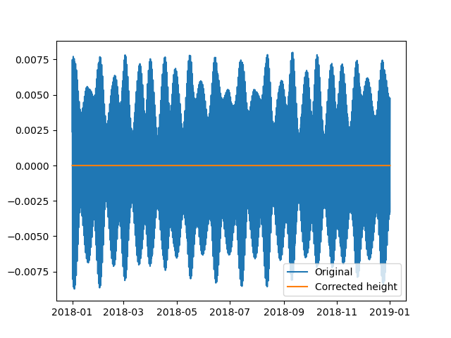
<matplotlib.legend.Legend object at 0x7f00b654d9d0>