Tidal Elevation Prediction using LPG Discretization

This example demonstrates how to use the model with LPG discretization to predict tidal elevation in a specified area of interest.

Warning

The model employed is an older FES tidal-atlas model due to its significantly smaller size compared to newer models. Do not use it for real applications. You can download the model from the AVISO website.

First, we import the required modules.

from __future__ import annotations

import os
import pathlib

import cartopy.crs
import matplotlib.pyplot
import numpy

import pyfes

First we create an environment variable to store the path to the model file. The configuration file is fully documented in the documentation.

Note

The content of the configuration file is viewable in the GitHub repository.

os.environ['DATASET_DIR'] = str(
    pathlib.Path().absolute().parent / 'tests' / 'python' / 'dataset'
)

config = pyfes.config.load(pathlib.Path().absolute() / 'fes_lpg.yml')

Please note that loading a global model can take up a lot of memory.

print(f'Model memory usage: {config.memory_usage() / 1e6:.2f} MB')

Model memory usage: 730.55 MB

config is a Configuration namedtuple that contains the tidal models and the runtime settings loaded from the configuration file.

print(config)

Configuration(models={'radial': TidalModelInterface(9 constituents, tide_type=RADIAL), 'tide': TidalModelInterface(10 constituents, tide_type=TIDE)}, settings=<FESSettings num_threads=0>)

Define the area of interest. Here we are interested in the area around the French coast.

LON_MIN = -5.0
LON_MAX = 10.0
LAT_MIN = 40.0
LAT_MAX = 55.0

Define the step size for the latitude and longitude grid.

LAT_STEP = 0.25
LON_STEP = 0.25

Define the interpolation quality flags.

UNDEFINED = 0
INTERPOLATED = 1
EXTRAPOLATED = 2

We can now create a grid to calculate the geocentric ocean tide around the French coast.

lons = numpy.arange(LON_MIN, LON_MAX + LON_STEP, LON_STEP)
lats = numpy.arange(LAT_MIN, LAT_MAX + LAT_STEP, LAT_STEP)
lons, lats = numpy.meshgrid(lons, lats)
shape = lons.shape
dates = numpy.full(shape, 'now', dtype='datetime64[us]')

We can now calculate the ocean tide and the radial tide.

tide, lp, lgp_flag = pyfes.evaluate_tide(
    config.models['tide'],
    dates.ravel(),
    lons.ravel(),
    lats.ravel(),
    settings=config.settings,
)
load, load_lp, _ = pyfes.evaluate_tide(
    config.models['radial'],
    dates.ravel(),
    lons.ravel(),
    lats.ravel(),
    settings=config.settings,
)

We can now calculate the geocentric ocean tide (as seen by a satellite).

geo_tide = tide + lp + load
geo_tide = geo_tide.reshape(lons.shape)

Mask the land values.

lgp_flag = lgp_flag.reshape(lons.shape)
geo_tide = numpy.ma.masked_where(lgp_flag == 0, geo_tide)

Create an interpolation quality flag array for visualization purposes.

flags = numpy.zeros(lgp_flag.shape, dtype=numpy.int8)
flags[lgp_flag > 0] = INTERPOLATED
flags[lgp_flag < 0] = EXTRAPOLATED

We can now plot the result.

fig = matplotlib.pyplot.figure(figsize=(15, 10))
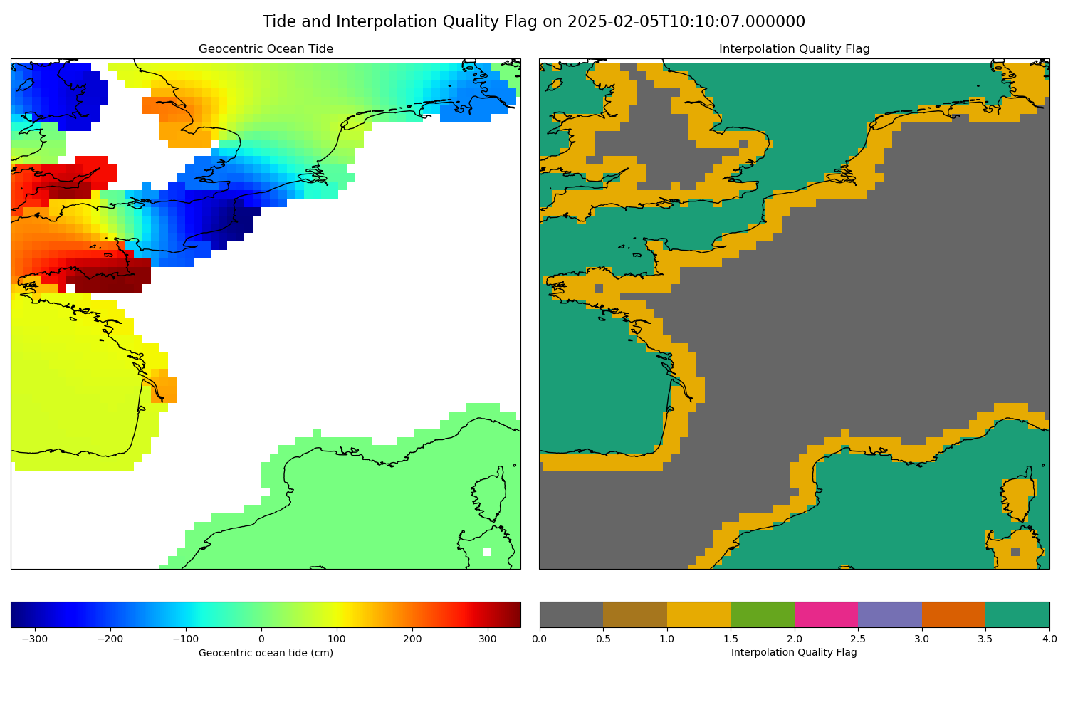
fig.suptitle(
    f'Tide and Interpolation Quality Flag on {dates[0, 0]}', fontsize=16
)

# Plot the geocentric ocean tide
ax1 = fig.add_subplot(1, 2, 1, projection=cartopy.crs.PlateCarree())
ax1.set_extent(
    [LON_MIN, LON_MAX, LAT_MIN, LAT_MAX], crs=cartopy.crs.PlateCarree()
)
ax1.coastlines()
ax1.set_title('Geocentric Ocean Tide')
ax1.set_xlabel('Longitude')
ax1.set_ylabel('Latitude')
mesh1 = ax1.pcolormesh(
    lons, lats, geo_tide, shading='auto', transform=cartopy.crs.PlateCarree()
)
colorbar1 = fig.colorbar(mesh1, ax=ax1, orientation='horizontal', pad=0.05)
colorbar1.set_label('Geocentric ocean tide (cm)')

# Plot the interpolation quality flag
ax2 = fig.add_subplot(1, 2, 2, projection=cartopy.crs.PlateCarree())
ax2.set_extent(
    [LON_MIN, LON_MAX, LAT_MIN, LAT_MAX], crs=cartopy.crs.PlateCarree()
)
ax2.coastlines()
ax2.set_title('Interpolation Quality Flag')
ax2.set_xlabel('Longitude')
ax2.set_ylabel('Latitude')
cmap = matplotlib.pyplot.get_cmap('Dark2_r', 3)
mesh2 = ax2.pcolormesh(
    lons,
    lats,
    flags,
    cmap=cmap,
    transform=cartopy.crs.PlateCarree(),
)
colorbar2 = fig.colorbar(
    mesh2,
    ax=ax2,
    orientation='horizontal',
    pad=0.05,
    ticks=[
        UNDEFINED,
        INTERPOLATED,
        EXTRAPOLATED,
    ],
)
colorbar2.set_ticklabels(
    [
        'Undefined',
        'Interpolated',
        'Extrapolated',
    ]
)
colorbar2.set_label('Interpolation Quality Flag')
fig.tight_layout()
matplotlib.pyplot.show()