Interpolation of LLC4320 ocean model

Interpolation of LLC4320 ocean model

The interpolation of this object is based on a R*Tree structure. To begin with, we start by building this object. By default, this object considers the WGS-84 geodetic coordinate system. But you can define another one using the class Spheroid.

import cartopy.crs
import cartopy.mpl.ticker
import intake
import matplotlib.pyplot
import numpy

import pyinterp

mesh = pyinterp.RTree()

Then, we will insert points into the tree. The class allows you to add points using two algorithms. The first one, called packing, will enable you to enter the values in the tree at once. This mechanism is the recommended solution to create an optimized in-memory structure, both in terms of construction time and queries. When this is not possible, you can insert new information into the tree as you go along using the insert method.

cat_url = ('https://raw.githubusercontent.com/pangeo-data/pangeo-datastore'
           '/master/intake-catalogs/ocean/llc4320.yaml')
cat = intake.open_catalog(cat_url)

Grid subsampling (original volume is too huge for this example)

indices = slice(0, None, 8)

Reads longitudes and latitudes of the grid

array = cat.LLC4320_grid.to_dask()
lons = array['XC'].isel(i=indices, j=indices)
lats = array['YC'].isel(i=indices, j=indices)

Reads SSH values for the first time step of the time series

ssh = cat.LLC4320_SSH.to_dask()
ssh = ssh['Eta'].isel(time=0, i=indices, j=indices)

Populates the search tree

mesh.packing(
    numpy.vstack((lons.values.ravel(), lats.values.ravel())).T,
    ssh.values.ravel())

When the tree is created, you can interpolate data with two algorithms:

• Inverse Distance Weighting or IDW

• Radial Basis Function or RBF

Yon can also search the nearest neighbors on the tree.

Note

When comparing an RBF to IDW, IDW will never predict values higher than the maximum measured value or lower than the minimum measured value. However, RBFs can predict values higher than the maximum values and lower than the minimum measured values.

In this example, we will under-sample the source grid at 1/32 degree over an area of the globe.

x0, x1 = 80, 170
y0, y1 = -45, 30
res = 1 / 32.0
mx, my = numpy.meshgrid(numpy.arange(x0, x1, res),
                        numpy.arange(y0, y1, res),
                        indexing='ij')

IDW interpolation

idw_eta, neighbors = mesh.inverse_distance_weighting(
    numpy.vstack((mx.ravel(), my.ravel())).T,
    within=True,  # Extrapolation is forbidden
    radius=55000,  # In a radius of 5.5 Km
    k=8,  # We are looking for at most 8 neighbours
    num_threads=0)
idw_eta = idw_eta.reshape(mx.shape)

RBF interpolation

rbf_eta, neighbors = mesh.radial_basis_function(
    numpy.vstack((mx.ravel(), my.ravel())).T,
    within=True,  # Extrapolation is forbidden
    k=11,  # We are looking for at most 11 neighbours
    num_threads=0)
rbf_eta = rbf_eta.reshape(mx.shape)

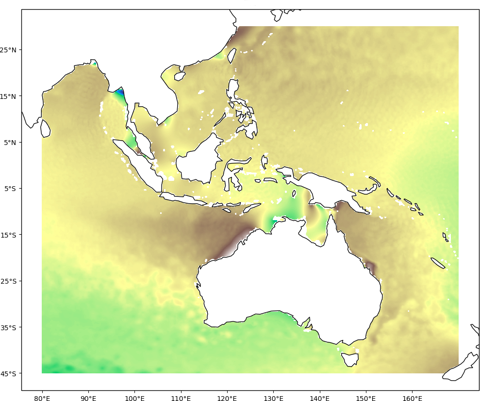
Let’s visualize our interpolated data

fig = matplotlib.pyplot.figure(figsize=(18, 9))
lon_formatter = cartopy.mpl.ticker.LongitudeFormatter(
    zero_direction_label=True)
lat_formatter = cartopy.mpl.ticker.LatitudeFormatter()
ax = fig.add_subplot(121, projection=cartopy.crs.PlateCarree())
ax.pcolormesh(mx,
              my,
              idw_eta,
              cmap='terrain',
              shading='auto',
              transform=cartopy.crs.PlateCarree())
ax.coastlines()
ax.xaxis.set_major_formatter(lon_formatter)
ax.yaxis.set_major_formatter(lat_formatter)
ax.set_xticks(numpy.arange(x0, x1, 10.0))
ax.set_yticks(numpy.arange(y0, y1, 10))
ax.set_title('Eta (IDW)')

ax = fig.add_subplot(122, projection=cartopy.crs.PlateCarree())
ax.pcolormesh(mx,
              my,
              rbf_eta,
              cmap='terrain',
              shading='auto',
              transform=cartopy.crs.PlateCarree())
ax.coastlines()
ax.xaxis.set_major_formatter(lon_formatter)
ax.yaxis.set_major_formatter(lat_formatter)
ax.set_xticks(numpy.arange(x0, x1, 10.0))
ax.set_yticks(numpy.arange(y0, y1, 10))
ax.set_title('Eta (RBF)')
fig.show()

The image below illustrates the result of the IDW interpolation: