Geometric Operations

This example demonstrates the geometric operations available in the pyinterp.geometry module. These operations allow you to transform, combine, and analyze geometric objects in various ways.

Operations Covered:

Set Operations:

Function	Description
union()	Combine geometries
intersection()	Find common areas
difference()	Subtract geometries

Transformation Operations:

Function	Description
simplify()	Reduce point count
densify()	Add intermediate points
convex_hull()	Minimum convex polygon
buffer()	Create buffer zones (Cartesian)

Validation and Correction:

Function	Description
is_valid()	Check validity
is_simple()	Check simplicity
correct()	Fix invalid geometries

Utility Operations:

Function	Description
reverse()	Reverse point order
unique()	Remove duplicate points
clear()	Clear geometry
convert_to_cartesian()	Convert coordinate systems
convert_to_geographic()	Convert back to geographic

Let’s start by importing the necessary libraries.

import matplotlib.pyplot
import numpy
from pyinterp.geometry import cartesian, geographic

Setup: Create Test Geometries

wgs84 = geographic.Spheroid()

# Create two overlapping polygons for set operations
poly1_lon = numpy.array([0.0, 0.0, 5.0, 5.0, 0.0], dtype=numpy.float64)
poly1_lat = numpy.array([0.0, 5.0, 5.0, 0.0, 0.0], dtype=numpy.float64)
poly1 = geographic.Polygon(geographic.Ring(poly1_lon, poly1_lat))

poly2_lon = numpy.array([3.0, 3.0, 8.0, 8.0, 3.0], dtype=numpy.float64)
poly2_lat = numpy.array([0.0, 5.0, 5.0, 0.0, 0.0], dtype=numpy.float64)
poly2 = geographic.Polygon(geographic.Ring(poly2_lon, poly2_lat))

print("Test geometries created")
print(
    f"Polygon 1 area: {geographic.algorithms.area(poly1, wgs84) * 1e-6:.4f} km²"
)
print(
    f"Polygon 2 area: {geographic.algorithms.area(poly2, wgs84) * 1e-6:.4f} km²"
)

Test geometries created
Polygon 1 area: 307541.8075 km²
Polygon 2 area: 307541.8075 km²

Set Operations: Union

The union() operation combines two geometries into one.

union_list = geographic.algorithms.union(poly1, poly2, spheroid=wgs84)
print(f"\nUnion operation returned {len(union_list)} polygon(s)")

if union_list:
    union_area = sum(geographic.algorithms.area(p, wgs84) for p in union_list)
    print(f"Union area: {union_area * 1e-6:.4f} km²")

    # Visualize the union
    print("Union polygon(s) created successfully")

Union operation returned 1 polygon(s)
Union area: 492104.3431 km²
Union polygon(s) created successfully

Set Operations: Intersection

The intersection() operation finds the common area between geometries.

intersection_list = geographic.algorithms.intersection(
    poly1, poly2, spheroid=wgs84
)
print(f"\nIntersection operation returned {len(intersection_list)} polygon(s)")

if intersection_list:
    intersection_area = sum(
        geographic.algorithms.area(p, wgs84) for p in intersection_list
    )
    print(f"Intersection area: {intersection_area * 1e-6:.4f} km²")

Intersection operation returned 1 polygon(s)
Intersection area: 122979.2793 km²

Set Operations: Difference

The difference() operation subtracts one geometry from another.

diff_list = geographic.algorithms.difference(poly1, poly2, spheroid=wgs84)
print(f"\nDifference operation returned {len(diff_list)} polygon(s)")

if diff_list:
    diff_area = sum(geographic.algorithms.area(p, wgs84) for p in diff_list)
    print(f"Difference (poly1 - poly2) area: {diff_area * 1e-6:.4f} km²")

    # Verify: poly1 area = intersection + difference
    poly1_area = geographic.algorithms.area(poly1, wgs84)
    expected_area = intersection_area + diff_area
    print(
        f"\nVerification: poly1 = {poly1_area * 1e-6:.4f} km², "
        f"intersection + difference = {expected_area * 1e-6:.4f} km²"
    )

Difference operation returned 1 polygon(s)
Difference (poly1 - poly2) area: 184562.5325 km²

Verification: poly1 = 307541.8075 km², intersection + difference = 307541.8118 km²

Simplification: Reducing Point Count

The simplify() operation reduces the number of points while preserving the overall shape.

# Create a dense line
dense_lon = numpy.linspace(0.0, 10.0, 100, dtype=numpy.float64)
dense_lat = numpy.sin(dense_lon * 0.5) + 45.0
dense_line = geographic.LineString(dense_lon, dense_lat)

print(f"\nOriginal line: {len(dense_line)} points")

# Simplify with different tolerances
simplified_10km = geographic.algorithms.simplify(
    dense_line, max_distance=10000.0, spheroid=wgs84
)
simplified_50km = geographic.algorithms.simplify(
    dense_line, max_distance=50000.0, spheroid=wgs84
)
simplified_100km = geographic.algorithms.simplify(
    dense_line, max_distance=100000.0, spheroid=wgs84
)

print(f"Simplified (10 km tolerance): {len(simplified_10km)} points")
print(f"Simplified (50 km tolerance): {len(simplified_50km)} points")
print(f"Simplified (100 km tolerance): {len(simplified_100km)} points")

Original line: 100 points
Simplified (10 km tolerance): 7 points
Simplified (50 km tolerance): 3 points
Simplified (100 km tolerance): 3 points

Densification: Adding Intermediate Points

The densify() operation adds intermediate points to ensure no segment is longer than a threshold.

# Create a sparse line
sparse_lon = numpy.array([0.0, 10.0], dtype=numpy.float64)
sparse_lat = numpy.array([0.0, 10.0], dtype=numpy.float64)
sparse_line = geographic.LineString(sparse_lon, sparse_lat)

print(f"\nOriginal sparse line: {len(sparse_line)} points")

# Densify with different max segment lengths
densified_100km = geographic.algorithms.densify(
    sparse_line, max_distance=100000.0, spheroid=wgs84
)
densified_50km = geographic.algorithms.densify(
    sparse_line, max_distance=50000.0, spheroid=wgs84
)

print(f"Densified (100 km segments): {len(densified_100km)} points")
print(f"Densified (50 km segments): {len(densified_50km)} points")

# Calculate the total length
length = geographic.algorithms.length(densified_100km, wgs84)
print(f"Total length: {length * 1e-3:.2f} km")

Original sparse line: 2 points
Densified (100 km segments): 17 points
Densified (50 km segments): 33 points
Total length: 1565.09 km

Convex Hull: Minimum Convex Polygon

The convex_hull() operation computes the smallest convex polygon containing all points.

# Create scattered points
points_lon = numpy.array([0.0, 1.0, 2.0, 1.0, 0.5], dtype=numpy.float64)
points_lat = numpy.array([0.0, 1.0, 0.0, -1.0, 0.5], dtype=numpy.float64)
points = geographic.MultiPoint(points_lon, points_lat)

hull = geographic.algorithms.convex_hull(points, spheroid=wgs84)

print("\nConvex Hull:")
print(f"  Input points: {len(points)}")
print(f"  Hull points: {geographic.algorithms.num_points(hull)}")
print(f"  Hull area: {geographic.algorithms.area(hull, wgs84) * 1e-6:.6f} km²")

Convex Hull:
  Input points: 5
  Hull points: 5
  Hull area: 24619.420408 km²

Closest Points: Finding Nearest Points

The closest_points() operation finds the nearest points between two geometries.

line1 = geographic.LineString(
    numpy.array([0.0, 2.0], dtype=numpy.float64),
    numpy.array([0.0, 0.0], dtype=numpy.float64),
)
line2 = geographic.LineString(
    numpy.array([5.0, 7.0], dtype=numpy.float64),
    numpy.array([1.0, 1.0], dtype=numpy.float64),
)

closest = geographic.algorithms.closest_points(line1, line2, spheroid=wgs84)
distance = geographic.algorithms.distance(closest.a, closest.b, spheroid=wgs84)

print("\nClosest points between two lines:")
print(f"  Point on line 1: ({closest.a.lon:.4f}, {closest.a.lat:.4f})")
print(f"  Point on line 2: ({closest.b.lon:.4f}, {closest.b.lat:.4f})")
print(f"  Distance: {distance * 1e-3:.3f} km")

Closest points between two lines:
  Point on line 1: (2.0000, 0.0000)
  Point on line 2: (5.0000, 1.0000)
  Distance: 351.771 km

Validation: Checking Geometry Validity

The is_valid() function checks if a geometry is topologically valid.

# Create a valid polygon
valid_lon = numpy.array([0.0, 2.0, 2.0, 0.0, 0.0], dtype=numpy.float64)
valid_lat = numpy.array([0.0, 0.0, 2.0, 2.0, 0.0], dtype=numpy.float64)
valid_poly = geographic.Polygon(geographic.Ring(valid_lon, valid_lat))

is_valid = geographic.algorithms.is_valid(valid_poly)
print(f"\nValid polygon is valid: {is_valid}")

# Create a self-intersecting (invalid) polygon
invalid_lon = numpy.array([0.0, 2.0, 2.0, 0.0, 0.0], dtype=numpy.float64)
invalid_lat = numpy.array([0.0, 0.0, 2.0, 2.0, 0.0], dtype=numpy.float64)
# Swap two points to create self-intersection
invalid_lon[2], invalid_lon[3] = invalid_lon[3], invalid_lon[2]
invalid_lat[2], invalid_lat[3] = invalid_lat[3], invalid_lat[2]

invalid_ring = geographic.Ring(invalid_lon, invalid_lat)
invalid_poly = geographic.Polygon(invalid_ring)

is_valid, reason = geographic.algorithms.is_valid(
    invalid_poly, return_reason=True
)
print(f"\nInvalid polygon is valid: {is_valid}")
if not is_valid:
    print(f"  Reason: {reason}")

Valid polygon is valid: False

Invalid polygon is valid: False
  Reason: Geometry has wrong orientation

Correction: Fixing Invalid Geometries

The correct() function attempts to fix invalid geometries.

print("\nCorrecting invalid polygon...")
geographic.algorithms.correct(invalid_poly)
is_valid_after = geographic.algorithms.is_valid(invalid_poly)
print(f"After correction, is valid: {is_valid_after}")

Correcting invalid polygon...
After correction, is valid: False

Simplicity: Checking for Self-Intersections

The is_simple() function checks if a geometry has no self-intersections.

simple_line = geographic.LineString(
    numpy.array([0.0, 1.0, 2.0], dtype=numpy.float64),
    numpy.array([0.0, 1.0, 2.0], dtype=numpy.float64),
)

print(
    f"\nSimple line is simple: {geographic.algorithms.is_simple(simple_line)}"
)
print(f"Simple line is valid: {geographic.algorithms.is_valid(simple_line)}")

Simple line is simple: True
Simple line is valid: True

Reverse: Reversing Point Order

The reverse() function reverses the order of points in a geometry.

original_line = geographic.LineString(
    numpy.array([0.0, 1.0, 2.0, 3.0], dtype=numpy.float64),
    numpy.array([0.0, 1.0, 2.0, 3.0], dtype=numpy.float64),
)

print("\nOriginal line points:")
for i, pt in enumerate(original_line):
    print(f"  {i}: ({pt.lon:.1f}, {pt.lat:.1f})")

# Reverse the line
geographic.algorithms.reverse(original_line)

print("After reversing:")
for i, pt in enumerate(original_line):
    print(f"  {i}: ({pt.lon:.1f}, {pt.lat:.1f})")

Original line points:
  0: (0.0, 0.0)
  1: (1.0, 1.0)
  2: (2.0, 2.0)
  3: (3.0, 3.0)
After reversing:
  0: (3.0, 3.0)
  1: (2.0, 2.0)
  2: (1.0, 1.0)
  3: (0.0, 0.0)

Unique: Removing Duplicate Points

The unique() function removes consecutive duplicate points.

duplicate_line = geographic.LineString(
    numpy.array([0.0, 1.0, 1.0, 2.0, 2.0, 2.0, 3.0], dtype=numpy.float64),
    numpy.array([0.0, 1.0, 1.0, 2.0, 2.0, 2.0, 3.0], dtype=numpy.float64),
)

print(f"\nLine with duplicates: {len(duplicate_line)} points")
geographic.algorithms.unique(duplicate_line)
print(f"After removing duplicates: {len(duplicate_line)} points")

Line with duplicates: 7 points
After removing duplicates: 4 points

Clear: Emptying Geometries

The clear() function removes all points from a geometry.

line_to_clear = geographic.LineString(
    numpy.array([0.0, 1.0, 2.0], dtype=numpy.float64),
    numpy.array([0.0, 1.0, 2.0], dtype=numpy.float64),
)

print(f"\nLine before clear: {len(line_to_clear)} points")
print(f"Is empty: {geographic.algorithms.is_empty(line_to_clear)}")

geographic.algorithms.clear(line_to_clear)

print(f"Line after clear: {len(line_to_clear)} points")
print(f"Is empty: {geographic.algorithms.is_empty(line_to_clear)}")

Line before clear: 3 points
Is empty: False
Line after clear: 0 points
Is empty: True

Coordinate System Conversion

Convert between geographic and cartesian coordinate systems.

geo_point = geographic.Point(10.0, 20.0)
cart_point = geographic.algorithms.convert_to_cartesian(geo_point)

print("\nGeographic to Cartesian:")
print(f"  Geographic: ({geo_point.lon}°, {geo_point.lat}°)")
print(f"  Cartesian: ({cart_point.x}, {cart_point.y})")

# Convert back
geo_from_cart = cartesian.algorithms.convert_to_geographic(cart_point)
print(f"  Back to geographic: ({geo_from_cart.lon}°, {geo_from_cart.lat}°)")

Geographic to Cartesian:
  Geographic: (10.0°, 20.0°)
  Cartesian: (10.0, 20.0)
  Back to geographic: (10.0°, 20.0°)

Convert a polygon

geo_ring_lon = numpy.array([0.0, 5.0, 5.0, 0.0, 0.0], dtype=numpy.float64)
geo_ring_lat = numpy.array([0.0, 0.0, 5.0, 5.0, 0.0], dtype=numpy.float64)
geo_ring = geographic.Ring(geo_ring_lon, geo_ring_lat)
geo_poly = geographic.Polygon(geo_ring)

cart_poly = geographic.algorithms.convert_to_cartesian(geo_poly)

geo_area = geographic.algorithms.area(geo_poly, wgs84)
cart_area = cartesian.algorithms.area(cart_poly)

print("\nPolygon conversion:")
print(f"  Geographic area: {geo_area * 1e-6:.2f} km²")
print(f"  Cartesian area: {cart_area:.2f} deg²")

Polygon conversion:
  Geographic area: -307541.81 km²
  Cartesian area: -25.00 deg²

Cartesian Buffer Operations

The cartesian geometry module provides buffer operations to create zones around geometries.

# Create a simple cartesian point
cart_pt = cartesian.Point(5.0, 5.0)

# Create buffer strategies
distance_symmetric = cartesian.algorithms.DistanceSymmetric(1.0)
join_round = cartesian.algorithms.JoinRound(points_per_circle=16)
end_round = cartesian.algorithms.EndRound(points_per_circle=16)
point_circle = cartesian.algorithms.PointCircle(points_per_circle=16)

# Create buffer around point
buffer_poly = cartesian.algorithms.buffer(
    cart_pt, distance_symmetric, join_round, end_round, point_circle
)

print("\nCartesian buffer:")
print(
    f"  Number of polygons in buffer: "
    f"{cartesian.algorithms.num_geometries(buffer_poly)}"
)
buffer_area = sum(cartesian.algorithms.area(p) for p in buffer_poly.polygons)
print(f"  Buffer area: {buffer_area:.4f} square units")
print(f"  Expected area (circle): {numpy.pi * 1.0**2:.4f} square units")

Cartesian buffer:
  Number of polygons in buffer: 1
  Buffer area: 3.0615 square units
  Expected area (circle): 3.1416 square units

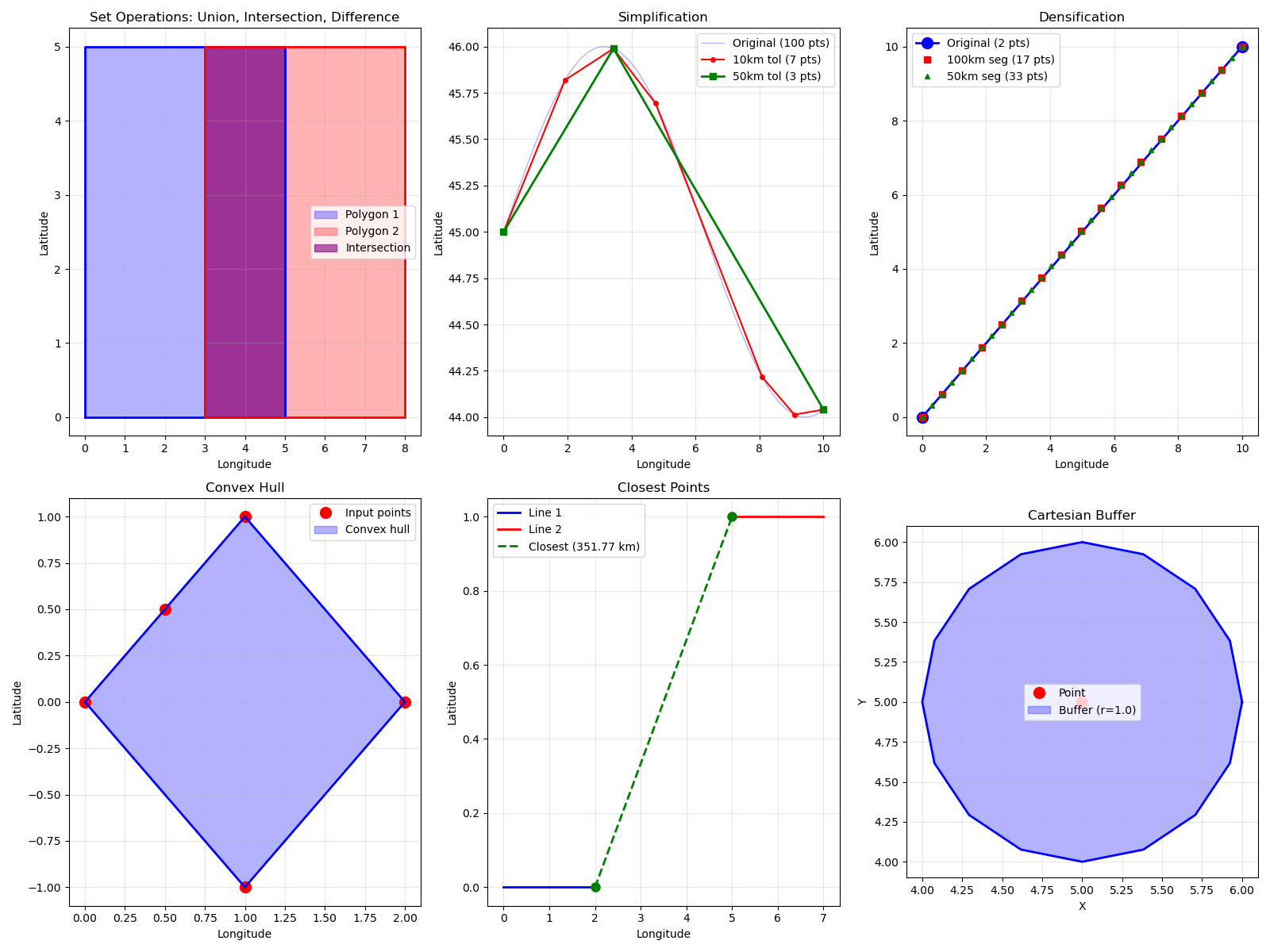
Visualization: Geometric Operations

fig = matplotlib.pyplot.figure(figsize=(16, 12))

# Plot 1: Set Operations
ax1 = fig.add_subplot(2, 3, 1)
ax1.fill(poly1_lon, poly1_lat, alpha=0.3, color="blue", label="Polygon 1")
ax1.plot(poly1_lon, poly1_lat, "b-", linewidth=2)
ax1.fill(poly2_lon, poly2_lat, alpha=0.3, color="red", label="Polygon 2")
ax1.plot(poly2_lon, poly2_lat, "r-", linewidth=2)

# Highlight intersection
if intersection_list:
    for poly in intersection_list:
        lons = [pt.lon for pt in poly.outer]
        lats = [pt.lat for pt in poly.outer]
        ax1.fill(lons, lats, alpha=0.6, color="purple", label="Intersection")

ax1.grid(True, alpha=0.3)
ax1.legend()
ax1.set_title("Set Operations: Union, Intersection, Difference")
ax1.set_xlabel("Longitude")
ax1.set_ylabel("Latitude")

# Plot 2: Simplification
ax2 = fig.add_subplot(2, 3, 2)
ax2.plot(
    *dense_line.to_arrays(),
    "b-",
    linewidth=1,
    alpha=0.3,
    label=f"Original ({len(dense_line)} pts)",
)
ax2.plot(
    *simplified_10km.to_arrays(),
    "ro-",
    markersize=4,
    linewidth=1.5,
    label=f"10km tol ({len(simplified_10km)} pts)",
)
ax2.plot(
    *simplified_50km.to_arrays(),
    "gs-",
    markersize=6,
    linewidth=2,
    label=f"50km tol ({len(simplified_50km)} pts)",
)
ax2.grid(True, alpha=0.3)
ax2.legend()
ax2.set_title("Simplification")
ax2.set_xlabel("Longitude")
ax2.set_ylabel("Latitude")

# Plot 3: Densification
ax3 = fig.add_subplot(2, 3, 3)
ax3.plot(
    *sparse_line.to_arrays(),
    "bo-",
    markersize=10,
    linewidth=2,
    label=f"Original ({len(sparse_line)} pts)",
)
ax3.plot(
    *densified_100km.to_arrays(),
    "rs",
    markersize=6,
    label=f"100km seg ({len(densified_100km)} pts)",
)
ax3.plot(
    *densified_50km.to_arrays(),
    "g^",
    markersize=4,
    label=f"50km seg ({len(densified_50km)} pts)",
)
ax3.grid(True, alpha=0.3)
ax3.legend()
ax3.set_title("Densification")
ax3.set_xlabel("Longitude")
ax3.set_ylabel("Latitude")

# Plot 4: Convex Hull
ax4 = fig.add_subplot(2, 3, 4)
ax4.plot(points_lon, points_lat, "ro", markersize=10, label="Input points")
hull_lons, hull_lats = hull.outer.to_arrays()
ax4.fill(hull_lons, hull_lats, alpha=0.3, color="blue", label="Convex hull")
ax4.plot(hull_lons, hull_lats, "b-", linewidth=2)
ax4.grid(True, alpha=0.3)
ax4.legend()
ax4.set_title("Convex Hull")
ax4.set_xlabel("Longitude")
ax4.set_ylabel("Latitude")

# Plot 5: Closest Points
ax5 = fig.add_subplot(2, 3, 5)
ax5.plot(
    *line1.to_arrays(),
    "b-",
    linewidth=2,
    label="Line 1",
)
ax5.plot(
    *line2.to_arrays(),
    "r-",
    linewidth=2,
    label="Line 2",
)
ax5.plot(
    *closest.to_arrays(),
    "g--",
    linewidth=2,
    label=f"Closest ({distance * 1e-3:.2f} km)",
)
ax5.plot(
    *closest.to_arrays(),
    "go",
    markersize=8,
)
ax5.grid(True, alpha=0.3)
ax5.legend()
ax5.set_title("Closest Points")
ax5.set_xlabel("Longitude")
ax5.set_ylabel("Latitude")

# Plot 6: Cartesian Buffer
ax6 = fig.add_subplot(2, 3, 6)
ax6.plot(cart_pt.x, cart_pt.y, "ro", markersize=10, label="Point")
for poly in buffer_poly.polygons:
    xs, ys = poly.outer.to_arrays()
    ax6.fill(xs, ys, alpha=0.3, color="blue", label="Buffer (r=1.0)")
    ax6.plot(xs, ys, "b-", linewidth=2)
# Only show label once
handles, labels = ax6.get_legend_handles_labels()
by_label = dict(zip(labels, handles, strict=False))
ax6.legend(by_label.values(), by_label.keys())
ax6.grid(True, alpha=0.3)
ax6.set_aspect("equal")
ax6.set_title("Cartesian Buffer")
ax6.set_xlabel("X")
ax6.set_ylabel("Y")

matplotlib.pyplot.tight_layout()