

Note
Go to the end to download the full example code or to run this example in your browser via Binder.
Advanced Geometric Features#
This example demonstrates advanced features of the pyinterp.geometry
module, including coordinate transformations, line interpolation, dateline
handling, spatial indexing, and performance comparisons.
Topics Covered:
Coordinate Transformations:
Coordinates: LLA to ECEF conversionTransformations between different spheroids
Line Operations:
line_interpolate():Get point at distance
curvilinear_distance():Distance along path
azimuth(): Forward bearing
Dateline Handling:
Creating and working with geometries crossing the International Date Line
Spatial Indexing:
RTree: Efficient spatial queries
Geodesic Strategies:
Let’s start by importing the necessary libraries.
import timeit

import cartopy.crs
import cartopy.feature
import matplotlib.pyplot
import numpy
from pyinterp.geometry import geographic
from pyinterp.core import config
Coordinate System Transformations#
The Coordinates class converts
between geodetic latitude, longitude, and altitude (LLA) and Earth-Centered,
Earth-Fixed (ECEF) coordinates.
wgs84 = geographic.Spheroid()
coords_wgs84 = geographic.Coordinates(wgs84)

# Generate random test points
generator = numpy.random.Generator(numpy.random.PCG64(0))
lon_samples = generator.uniform(-180.0, 180.0, 100_000)
lat_samples = generator.uniform(-90.0, 90.0, 100_000)
alt_samples = generator.uniform(-10_000, 100_000, 100_000)

print("Coordinate Transformations:")
print(f"  Converting {len(lon_samples)} points to ECEF...")

# Convert to ECEF
x, y, z = coords_wgs84.lla_to_ecef(
    lon_samples, lat_samples, alt_samples, num_threads=0
)
print(f"  X range: [{x.min():.2f}, {x.max():.2f}] m")
print(f"  Y range: [{y.min():.2f}, {y.max():.2f}] m")
print(f"  Z range: [{z.min():.2f}, {z.max():.2f}] m")

# Convert back to LLA
lon_restored, lat_restored, alt_restored = coords_wgs84.ecef_to_lla(
    x, y, z, num_threads=0
)

# Check round-trip accuracy
lon_error = numpy.abs(lon_samples - lon_restored).max()
lat_error = numpy.abs(lat_samples - lat_restored).max()
alt_error = numpy.abs(alt_samples - alt_restored).max()

print("\nRound-trip errors:")
print(f"  Longitude: {lon_error:.2e} degrees")
print(f"  Latitude: {lat_error:.2e} degrees")
print(f"  Altitude: {alt_error:.2e} m")
Coordinate Transformations:
  Converting 100000 points to ECEF...
  X range: [-6473791.46, 6475418.84] m
  Y range: [-6476146.88, 6467975.51] m
  Z range: [-6456397.08, 6456273.14] m

Round-trip errors:
  Longitude: 2.84e-14 degrees
  Latitude: 2.84e-14 degrees
  Altitude: 4.07e-09 m
Transforming Between Different Spheroids#
You can transform coordinates between different reference ellipsoids.
grs80 = geographic.Spheroid(6378137.0, 1 / 298.257222101)
coords_grs80 = geographic.Coordinates(grs80)

# Transform from WGS84 to GRS80
lon_grs80, lat_grs80, alt_grs80 = coords_wgs84.transform(
    coords_grs80,
    lon_samples[:1000],
    lat_samples[:1000],
    alt_samples[:1000],
    num_threads=0,
)

# Compute differences
lon_diff = numpy.abs(lon_samples[:1000] - lon_grs80).max()
lat_diff = numpy.abs(lat_samples[:1000] - lat_grs80).max()
alt_diff = numpy.abs(alt_samples[:1000] - alt_grs80).max()

print("\nWGS84 to GRS80 transformation differences:")
print(f"  Longitude: {lon_diff:.2e} degrees")
print(f"  Latitude: {lat_diff:.2e} degrees")
print(f"  Altitude: {alt_diff:.2e} m")
WGS84 to GRS80 transformation differences:
  Longitude: 2.84e-14 degrees
  Latitude: 9.43e-10 degrees
  Altitude: 1.05e-04 m
Benchmark transformations
elapsed = timeit.timeit(
    lambda: coords_wgs84.transform(
        coords_grs80,
        lon_samples[:1000],
        lat_samples[:1000],
        alt_samples[:1000],
        num_threads=0,
    ),
    number=10,
)
print(f"\nTransformation time (1000 points, 10 runs): {elapsed:.6f} seconds")
print(f"Average time per run: {elapsed / 10:.6f} seconds")
Transformation time (1000 points, 10 runs): 0.010419 seconds
Average time per run: 0.001042 seconds
Line Interpolation: Getting Points at Specific Distances#
The line_interpolate()
function returns a point at a specified distance along a line.
# Create a path from Paris to New York
paris = geographic.Point(2.3488, 48.8534)
new_york = geographic.Point(-73.9385, 40.6643)

path = geographic.LineString(
    numpy.array([paris.lon, new_york.lon], dtype=numpy.float64),
    numpy.array([paris.lat, new_york.lat], dtype=numpy.float64),
)

# Get the total distance
total_distance = geographic.algorithms.length(path, spheroid=wgs84)
print("\nPath from Paris to New York:")
print(f"  Total distance: {total_distance * 1e-3:.2f} km")

# Interpolate points at regular intervals
num_waypoints = 10
waypoints = []
for i in range(num_waypoints + 1):
    distance = (total_distance * i) / num_waypoints
    waypoint = geographic.algorithms.line_interpolate(
        path, distance, spheroid=wgs84
    )
    waypoints.append(waypoint)
    print(
        f"  Waypoint {i}: ({waypoint.lon:.4f}, {waypoint.lat:.4f}) "
        f"at {distance * 1e-3:.2f} km"
    )
Path from Paris to New York:
  Total distance: 5851.42 km
  Waypoint 0: (2.3488, 48.8534) at 0.00 km
  Waypoint 1: (-5.3328, 50.5528) at 585.14 km
  Waypoint 2: (-13.4918, 51.7114) at 1170.28 km
  Waypoint 3: (-21.9662, 52.2787) at 1755.42 km
  Waypoint 4: (-30.5393, 52.2276) at 2340.57 km
  Waypoint 5: (-38.9757, 51.5607) at 2925.71 km
  Waypoint 6: (-47.0656, 50.3093) at 3510.85 km
  Waypoint 7: (-54.6582, 48.5271) at 4095.99 km
  Waypoint 8: (-61.6727, 46.2801) at 4681.13 km
  Waypoint 9: (-68.0908, 43.6373) at 5266.27 km
  Waypoint 10: (-73.9384, 40.6642) at 5851.42 km
Curvilinear Distance: Distance Along a Path#
The curvilinear_distance()
function computes the cumulative distance from the start of a line.
# Create a more complex path
lon_path = numpy.array([0.0, 1.0, 2.0, 3.0, 4.0], dtype=numpy.float64)
lat_path = numpy.array([0.0, 1.0, 0.5, 1.5, 1.0], dtype=numpy.float64)
complex_path = geographic.LineString(lon_path, lat_path)

curv_distances = geographic.algorithms.curvilinear_distance(
    complex_path, spheroid=wgs84
)

print("\nCurvilinear distances along path:")
for i, (lon, lat, dist) in enumerate(
    zip(lon_path, lat_path, curv_distances, strict=False)
):
    print(
        f"  Point {i} ({lon:.2f}, {lat:.2f}): {dist * 1e-3:.3f} km from start"
    )
Curvilinear distances along path:
  Point 0 (0.00, 0.00): 0.000 km from start
  Point 1 (1.00, 1.00): 156.898 km from start
  Point 2 (2.00, 0.50): 281.181 km from start
  Point 3 (3.00, 1.50): 438.070 km from start
  Point 4 (4.00, 1.00): 562.338 km from start
Azimuth: Forward Bearing Between Points#
The azimuth() function
computes the forward bearing from one point to another.
azimuth_pny = geographic.algorithms.azimuth(
    paris, new_york, spheroid=wgs84, strategy=geographic.algorithms.VINCENTY
)
azimuth_nyp = geographic.algorithms.azimuth(
    new_york, paris, spheroid=wgs84, strategy=geographic.algorithms.VINCENTY
)

print("\nAzimuth calculations:")
print(f"  Paris to New York: {numpy.degrees(azimuth_pny):.2f}°")
print(f"  New York to Paris: {numpy.degrees(azimuth_nyp):.2f}°")

# Note: Forward and backward azimuths are not simply 180° apart on a sphere
difference = abs(
    numpy.degrees(azimuth_pny) - (numpy.degrees(azimuth_nyp) - 180)
)
print(f"  Difference from 180°: {difference:.2f}°")
Azimuth calculations:
  Paris to New York: -68.26°
  New York to Paris: 53.72°
  Difference from 180°: 58.02°
Handling the International Date Line#
Geographic boxes and geometries that span the International Date Line (180°/-180° longitude) require special handling.
# Create a box that crosses the dateline
dateline_box = geographic.Box((170.0, -30.0), (-170.0, 30.0))

print("\nDateline-crossing box:")
print(
    f"  Min corner: ({dateline_box.min_corner.lon}, "
    f"{dateline_box.min_corner.lat})"
)
print(
    f"  Max corner: ({dateline_box.max_corner.lon}, "
    f"{dateline_box.max_corner.lat})"
)
Dateline-crossing box:
  Min corner: (170.0, -30.0)
  Max corner: (190.0, 30.0)
Test points around the dateline
test_points = [
    (170, 0, "Left edge (170°E)"),
    (175, 0, "Eastern section (175°E)"),
    (180, 10, "On dateline (180°)"),
    (-180, -10, "On dateline (-180°)"),
    (-175, 0, "Western section (-175°W)"),
    (-170, 0, "Right edge (-170°W)"),
    (0, 0, "Prime meridian (outside)"),
    (160, 0, "West of box (160°E)"),
    (-160, 0, "East of box (-160°W)"),
]

print("\nPoint-in-box tests:")
print(f"{'Longitude':>10} {'Latitude':>10} {'Within?':>10} {'Description'}")
print("-" * 70)

for lon, lat, description in test_points:
    point = geographic.Point(lon, lat)
    is_inside = geographic.algorithms.within(point, dateline_box)
    status = "Yes" if is_inside else "No"
    print(f"{lon:>10.1f} {lat:>10.1f} {status:>10}  {description}")
Point-in-box tests:
 Longitude   Latitude    Within? Description
----------------------------------------------------------------------
     170.0        0.0         No  Left edge (170°E)
     175.0        0.0        Yes  Eastern section (175°E)
     180.0       10.0        Yes  On dateline (180°)
    -180.0      -10.0        Yes  On dateline (-180°)
    -175.0        0.0        Yes  Western section (-175°W)
    -170.0        0.0         No  Right edge (-170°W)
       0.0        0.0         No  Prime meridian (outside)
     160.0        0.0         No  West of box (160°E)
    -160.0        0.0         No  East of box (-160°W)
RTree Spatial Indexing#
The RTree class provides efficient
spatial indexing for fast nearest-neighbor queries.
# Create an RTree and populate it with random points
rtree = geographic.RTree()

# Generate random data
n_points = 10_000
data_lon = generator.uniform(-180.0, 180.0, n_points)
data_lat = generator.uniform(-60.0, 60.0, n_points)
data_values = generator.uniform(0.0, 100.0, n_points)

# Create coordinate array (lon, lat)
coordinates = numpy.column_stack([data_lon, data_lat])

# Insert into RTree
rtree.insert(coordinates, data_values)

print("\nRTree Spatial Index:")
print(f"  Indexed points: {rtree.size()}")
print(f"  Is empty: {rtree.empty()}")

# Get bounds
bounds = rtree.bounds()
if bounds:
    min_bounds, max_bounds = bounds
    print(
        f"  Bounds: ({min_bounds[0]:.2f}, {min_bounds[1]:.2f}) to "
        f"({max_bounds[0]:.2f}, {max_bounds[1]:.2f})"
    )
RTree Spatial Index:
  Indexed points: 10000
  Is empty: False
  Bounds: (-180.00, -60.00) to (180.00, 59.99)
Query nearest neighbors
query_points = numpy.array(
    [[0.0, 0.0], [45.0, 45.0], [-120.0, 30.0]], dtype=numpy.float64
)

settings = config.rtree.Query()

# Query the RTree
distances, values = rtree.query(query_points, settings)

print("\nNearest neighbor queries:")
for i, (qlon, qlat) in enumerate(query_points):
    print(f"  Query point ({qlon}, {qlat}):")
    for j, (dist, val) in enumerate(
        zip(distances[i], values[i], strict=False)
    ):
        if not numpy.isnan(dist):
            print(
                f"    Neighbor {j}: distance={dist * 1e-3:.2f} km, "
                f"value={val:.2f}"
            )
Nearest neighbor queries:
  Query point (0.0, 0.0):
    Neighbor 0: distance=98.45 km, value=86.00
    Neighbor 1: distance=107.51 km, value=27.11
    Neighbor 2: distance=175.07 km, value=25.24
    Neighbor 3: distance=209.22 km, value=7.36
    Neighbor 4: distance=256.15 km, value=79.94
    Neighbor 5: distance=266.47 km, value=35.39
    Neighbor 6: distance=272.78 km, value=97.55
    Neighbor 7: distance=281.96 km, value=42.04
  Query point (45.0, 45.0):
    Neighbor 0: distance=69.48 km, value=83.78
    Neighbor 1: distance=104.53 km, value=39.88
    Neighbor 2: distance=107.08 km, value=47.61
    Neighbor 3: distance=151.05 km, value=55.43
    Neighbor 4: distance=168.51 km, value=60.57
    Neighbor 5: distance=180.96 km, value=72.21
    Neighbor 6: distance=237.06 km, value=61.89
    Neighbor 7: distance=276.98 km, value=13.04
  Query point (-120.0, 30.0):
    Neighbor 0: distance=58.70 km, value=73.69
    Neighbor 1: distance=237.77 km, value=46.14
    Neighbor 2: distance=268.35 km, value=17.99
    Neighbor 3: distance=286.30 km, value=20.71
    Neighbor 4: distance=290.66 km, value=87.29
    Neighbor 5: distance=292.54 km, value=23.18
    Neighbor 6: distance=294.91 km, value=74.25
    Neighbor 7: distance=309.41 km, value=60.48
Geodesic Strategy Performance Comparison#
Different geodesic calculation strategies offer different trade-offs between accuracy and performance.
# Test points
london = geographic.Point(-0.1276, 51.5074)
tokyo = geographic.Point(139.6917, 35.6895)

strategies = [
    (geographic.algorithms.ANDOYER, "ANDOYER"),
    (geographic.algorithms.THOMAS, "THOMAS"),
    (geographic.algorithms.VINCENTY, "VINCENTY"),
    (geographic.algorithms.KARNEY, "KARNEY"),
]

print("\nGeodesic strategy comparison (London to Tokyo):")
print(f"{'Strategy':<15} {'Distance (km)':<15} {'Time (µs)':<15}")
print("-" * 50)

for strategy, name in strategies:
    # Calculate distance
    distance = geographic.algorithms.distance(
        london, tokyo, spheroid=wgs84, strategy=strategy
    )

    # Benchmark
    elapsed = timeit.timeit(
        lambda strategy=strategy: geographic.algorithms.distance(
            london, tokyo, spheroid=wgs84, strategy=strategy
        ),
        number=1000,
    )
    time_per_call = (elapsed / 1000) * 1e6  # Convert to microseconds

    print(f"{name:<15} {distance * 1e-3:<15.3f} {time_per_call:<15.3f}")
Geodesic strategy comparison (London to Tokyo):
Strategy        Distance (km)   Time (µs)
--------------------------------------------------
ANDOYER         9582.297        0.216
THOMAS          9582.302        0.254
VINCENTY        9582.302        0.482
KARNEY          19993.535       13.385
Azimuth calculation with different strategies
print("\nAzimuth calculation (London to Tokyo):")
print(f"{'Strategy':<15} {'Azimuth (degrees)':<20}")
print("-" * 40)

for strategy, name in strategies:
    azimuth = geographic.algorithms.azimuth(
        london, tokyo, spheroid=wgs84, strategy=strategy
    )
    print(f"{name:<15} {numpy.degrees(azimuth):<20.6f}")
Azimuth calculation (London to Tokyo):
Strategy        Azimuth (degrees)
----------------------------------------
ANDOYER         31.653401
THOMAS          31.653339
VINCENTY        31.653339
KARNEY          119.294357
Spheroid Properties#
Explore various properties of reference ellipsoids.
print("\nSpheroid properties comparison:")
print(f"{'Property':<35} {'WGS84':<20} {'GRS80':<20}")
print("-" * 75)

properties = [
    ("Semi-major axis (m)", lambda s: f"{s.semi_major_axis:,.2f}"),
    ("Flattening", lambda s: f"{s.flattening:.10f}"),
    ("Semi-minor axis (m)", lambda s: f"{s.semi_minor_axis():,.2f}"),
    ("Mean radius (m)", lambda s: f"{s.mean_radius():,.2f}"),
    ("Authalic radius (m)", lambda s: f"{s.authalic_radius():,.2f}"),
    ("Volumetric radius (m)", lambda s: f"{s.volumetric_radius():,.2f}"),
    (
        "Equatorial circumference (m)",
        lambda s: f"{s.equatorial_circumference():,.2f}",
    ),
    (
        "First eccentricity squared",
        lambda s: f"{s.first_eccentricity_squared():.10f}",
    ),
    (
        "Second eccentricity squared",
        lambda s: f"{s.second_eccentricity_squared():.10f}",
    ),
]

for prop_name, prop_func in properties:
    wgs84_val = prop_func(wgs84)
    grs80_val = prop_func(grs80)
    print(f"{prop_name:<35} {wgs84_val:<20} {grs80_val:<20}")
Spheroid properties comparison:
Property                            WGS84                GRS80
---------------------------------------------------------------------------
Semi-major axis (m)                 6,378,137.00         6,378,137.00
Flattening                          0.0033528107         0.0033528107
Semi-minor axis (m)                 6,356,752.31         6,356,752.31
Mean radius (m)                     6,371,008.77         6,371,008.77
Authalic radius (m)                 6,371,007.18         6,371,007.18
Volumetric radius (m)               6,371,000.79         6,371,000.79
Equatorial circumference (m)        40,075,016.69        40,075,016.69
First eccentricity squared          0.0066943800         0.0066943800
Second eccentricity squared         0.0067394967         0.0067394968
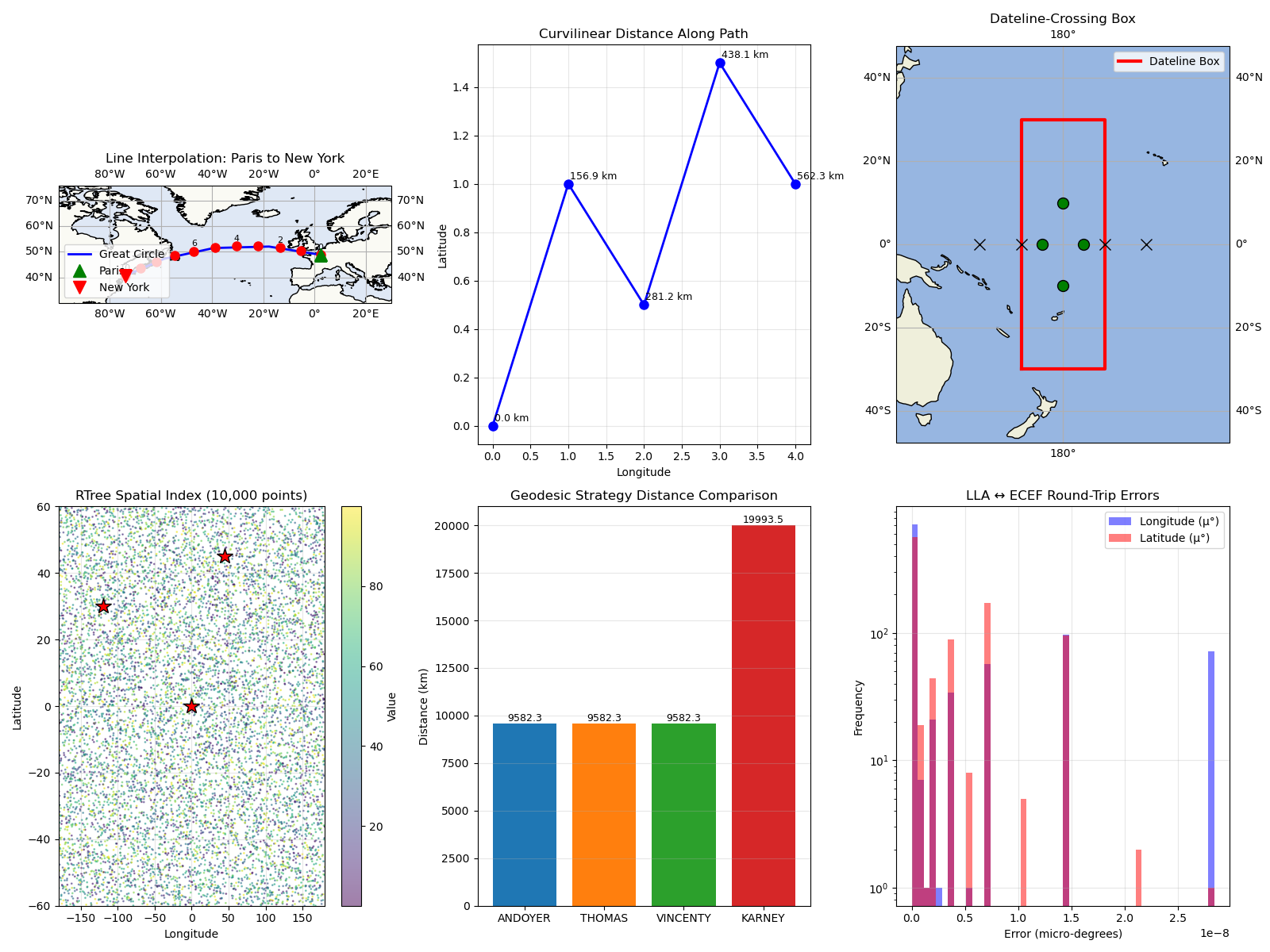
Visualization: Advanced Features#
fig = matplotlib.pyplot.figure(figsize=(16, 12))

# Plot 1: Line interpolation waypoints
ax1 = fig.add_subplot(2, 3, 1, projection=cartopy.crs.PlateCarree())
ax1.add_feature(cartopy.feature.LAND, alpha=0.3)
ax1.add_feature(cartopy.feature.OCEAN, alpha=0.3)
ax1.add_feature(cartopy.feature.COASTLINE)
ax1.gridlines(draw_labels=True, dms=True, x_inline=False, y_inline=False)
ax1.set_extent([-100, 30, 30, 60])

# Plot the great circle path
ax1.plot(
    [paris.lon, new_york.lon],
    [paris.lat, new_york.lat],
    "b-",
    linewidth=2,
    label="Great Circle",
    transform=cartopy.crs.Geodetic(),
)

# Plot waypoints
for i, wp in enumerate(waypoints):
    ax1.plot(
        wp.lon,
        wp.lat,
        "ro",
        markersize=8,
        transform=cartopy.crs.PlateCarree(),
        zorder=5,
    )
    if i % 2 == 0:  # Label every other waypoint
        ax1.text(
            wp.lon,
            wp.lat + 2,
            f"{i}",
            transform=cartopy.crs.PlateCarree(),
            fontsize=8,
            ha="center",
        )

ax1.plot(
    paris.lon,
    paris.lat,
    "g^",
    markersize=12,
    label="Paris",
    transform=cartopy.crs.PlateCarree(),
    zorder=6,
)
ax1.plot(
    new_york.lon,
    new_york.lat,
    "rv",
    markersize=12,
    label="New York",
    transform=cartopy.crs.PlateCarree(),
    zorder=6,
)

ax1.legend(loc="lower left")
ax1.set_title("Line Interpolation: Paris to New York")

# Plot 2: Curvilinear distance
ax2 = fig.add_subplot(2, 3, 2)
ax2.plot(lon_path, lat_path, "bo-", linewidth=2, markersize=8)
for lon, lat, dist in zip(lon_path, lat_path, curv_distances, strict=False):
    ax2.text(
        lon + 0.02,
        lat + 0.02,
        f"{dist * 1e-3:.1f} km",
        fontsize=9,
    )
ax2.grid(True, alpha=0.3)
ax2.set_xlabel("Longitude")
ax2.set_ylabel("Latitude")
ax2.set_title("Curvilinear Distance Along Path")

# Plot 3: Dateline-crossing box
ax3 = fig.add_subplot(
    2, 3, 3, projection=cartopy.crs.PlateCarree(central_longitude=180)
)
ax3.add_feature(cartopy.feature.LAND)
ax3.add_feature(cartopy.feature.OCEAN)
ax3.add_feature(cartopy.feature.COASTLINE)
ax3.gridlines(draw_labels=True, dms=True, x_inline=False, y_inline=False)
ax3.set_extent([140, -140, -40, 40])

# Plot the box boundaries (need to handle dateline wrapping)
box_lon = [170, 190, 190, 170, 170]  # 190 = -170 + 360
box_lat = [-30, -30, 30, 30, -30]
ax3.plot(
    box_lon,
    box_lat,
    color="red",
    linewidth=3,
    transform=cartopy.crs.Geodetic(),
    label="Dateline Box",
)

# Plot test points
for lon, lat, _ in test_points:
    point = geographic.Point(lon, lat)
    is_inside = geographic.algorithms.within(point, dateline_box)
    color = "green" if is_inside else "gray"
    marker = "o" if is_inside else "x"
    ax3.plot(
        lon,
        lat,
        marker,
        color=color,
        markersize=10,
        markeredgecolor="black",
        markeredgewidth=1,
        transform=cartopy.crs.PlateCarree(),
    )

ax3.legend()
ax3.set_title("Dateline-Crossing Box")

# Plot 4: RTree spatial index
ax4 = fig.add_subplot(2, 3, 4)
scatter = ax4.scatter(
    data_lon, data_lat, c=data_values, s=1, cmap="viridis", alpha=0.5
)
matplotlib.pyplot.colorbar(scatter, ax=ax4, label="Value")

# Plot query points and their nearest neighbors
for qlon, qlat in query_points:
    ax4.plot(
        qlon,
        qlat,
        "r*",
        markersize=15,
        markeredgecolor="black",
        markeredgewidth=1,
    )

ax4.grid(True, alpha=0.3)
ax4.set_xlabel("Longitude")
ax4.set_ylabel("Latitude")
ax4.set_title(f"RTree Spatial Index ({n_points:,} points)")
ax4.set_xlim(-180, 180)
ax4.set_ylim(-60, 60)

# Plot 5: Geodesic strategy comparison
ax5 = fig.add_subplot(2, 3, 5)
strategy_names = [name for _, name in strategies]
distances_km = [
    geographic.algorithms.distance(
        london, tokyo, spheroid=wgs84, strategy=strategy
    )
    * 1e-3
    for strategy, _ in strategies
]

bars = ax5.bar(
    strategy_names,
    distances_km,
    color=["#1f77b4", "#ff7f0e", "#2ca02c", "#d62728"],
)
ax5.set_ylabel("Distance (km)")
ax5.set_title("Geodesic Strategy Distance Comparison")
ax5.grid(True, alpha=0.3, axis="y")

# Add value labels on bars
for bar, dist in zip(bars, distances_km, strict=False):
    height = bar.get_height()
    ax5.text(
        bar.get_x() + bar.get_width() / 2.0,
        height,
        f"{dist:.1f}",
        ha="center",
        va="bottom",
        fontsize=9,
    )

# Plot 6: Coordinate transformation accuracy
ax6 = fig.add_subplot(2, 3, 6)

# Sample a subset for visualization
rng = numpy.random.default_rng(42)
sample_size = 1000
sample_indices = rng.choice(len(lon_samples), sample_size, replace=False)

lon_sample = lon_samples[sample_indices]
lat_sample = lat_samples[sample_indices]
alt_sample = alt_samples[sample_indices]
# Transform to ECEF and back
x_s, y_s, z_s = coords_wgs84.lla_to_ecef(
    lon_sample, lat_sample, alt_sample, num_threads=0
)
lon_s, lat_s, alt_s = coords_wgs84.ecef_to_lla(x_s, y_s, z_s, num_threads=0)

# Calculate errors
lon_err = numpy.abs(lon_sample - lon_s) * 1e6  # Convert to micro-degrees
lat_err = numpy.abs(lat_sample - lat_s) * 1e6
alt_err = numpy.abs(alt_sample - alt_s)  # Keep in meters

# Plot error distributions
ax6.hist(lon_err, bins=50, alpha=0.5, label="Longitude (µ°)", color="blue")
ax6.hist(lat_err, bins=50, alpha=0.5, label="Latitude (µ°)", color="red")
ax6.set_xlabel("Error (micro-degrees)")
ax6.set_ylabel("Frequency")
ax6.set_title("LLA ↔ ECEF Round-Trip Errors")
ax6.legend()
ax6.grid(True, alpha=0.3)
ax6.set_yscale("log")

matplotlib.pyplot.tight_layout()
Total running time of the script: (0 minutes 1.799 seconds)