

Note
Go to the end to download the full example code or to run this example in your browser via Binder.
Track Decomposition#
This example demonstrates how to use
decompose_track() to split a satellite
ground track into meaningful segments. The function supports two strategies:
"latitude_bands"— fixed latitude thresholds producing up to three zones (south polar, mid-latitude, north polar). Backward-compatible with the originalcreate_processing_blocksbehaviour."monotonic"— splits at every latitude direction change (ascending ↔ descending), producing tight bounding boxes for near-polar orbits.
We build a realistic track by propagating several consecutive passes from a SWOT-like ephemeris, then explore the decomposition options.
import pathlib

import cartopy.crs as ccrs
import matplotlib.patches as mpatches
import matplotlib.pyplot as plt
import numpy as np

import pyinterp.orbit
import pyinterp.tests
from pyinterp.geometry import satellite
Loading the Ephemeris#
Reuse the helper from the orbit example to load the test ephemeris file.
def load_test_ephemeris(
    filename: pathlib.Path,
) -> tuple[float, np.ndarray, np.ndarray, np.ndarray, np.timedelta64]:
    """Load the ephemeris from a text file."""
    with open(filename, encoding="utf-8") as stream:
        lines = stream.readlines()

    def to_dict(comments: list[str]) -> dict[str, float]:
        result = {}
        for item in comments:
            if not item.startswith("#"):
                raise ValueError("Comments must start with #")
            key, value = item[1:].split("=")
            result[key.strip()] = float(value)
        return result

    settings = to_dict(lines[:2])
    del lines[:2]

    ephemeris = np.loadtxt(
        lines,
        delimiter=" ",
        dtype={
            "names": ("time", "longitude", "latitude", "height"),
            "formats": ("f8", "f8", "f8", "f8"),
        },
    )
    return (
        settings["height"],
        ephemeris["longitude"],
        ephemeris["latitude"],
        ephemeris["time"].astype("timedelta64[s]"),
        np.timedelta64(int(settings["cycle_duration"] * 86400.0 * 1e9), "ns"),
    )
Building a Realistic Multi-Pass Track#
Compute the orbit and concatenate several consecutive nadir tracks so the resulting ground track spans all latitude zones.
orbit = pyinterp.orbit.calculate_orbit(
    *load_test_ephemeris(pyinterp.tests.ephemeris_path())
)

n_passes = 6  # six half-orbit arcs ≈ three full revolutions
lon_parts, lat_parts = [], []
for pass_number in range(1, n_passes + 1):
    pass_ = pyinterp.orbit.calculate_pass(pass_number, orbit)
    if pass_ is None:
        continue
    lon_parts.append(pass_.lon_nadir)
    lat_parts.append(pass_.lat_nadir)

lon = np.concatenate(lon_parts)
lat = np.concatenate(lat_parts)

print(f"Concatenated track : {len(lon)} points over {n_passes} passes")
print(f"Longitude range    : [{lon.min():.1f}°, {lon.max():.1f}°]")
print(f"Latitude range     : [{lat.min():.1f}°, {lat.max():.1f}°]")
Concatenated track : 54158 points over 6 passes
Longitude range    : [-180.0°, 180.0°]
Latitude range     : [-77.5°, 77.7°]
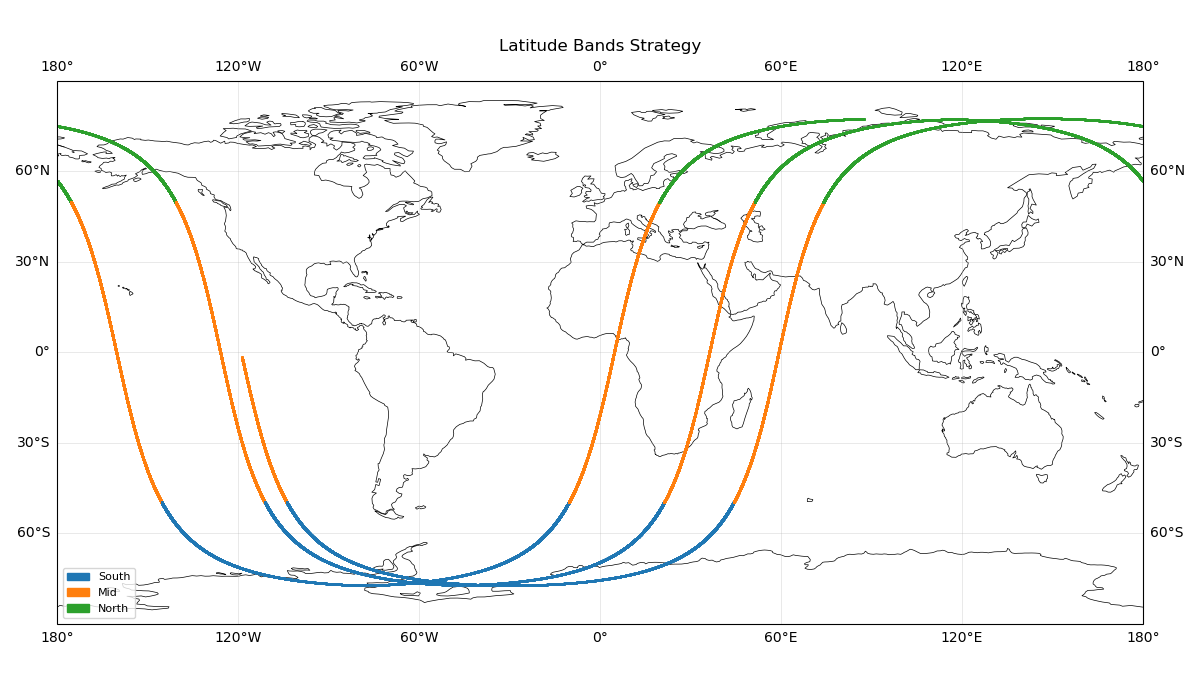
Decomposing with Latitude Bands#
The "latitude_bands" strategy divides the track at the south and north
latitude thresholds (default −50° / +50°). Each segment is labelled with its
dominant LatitudeZone and
OrbitDirection.
segments_bands = satellite.decompose_track(lon, lat, strategy="latitude_bands")

print(f"\nLatitude-bands strategy → {len(segments_bands)} segment(s)")
for seg in segments_bands:
    print(f"  {seg}")
Latitude-bands strategy → 12 segment(s)
  TrackSegment([0, 2771], zone=mid, orbit=prograde, bbox=lon[-118.71,-103.85] lat[-50.00,-1.72])
  TrackSegment([2772, 7019], zone=south, orbit=prograde, bbox=lon[-103.85,44.29] lat[-77.50,-50.01])
  TrackSegment([7020, 12748], zone=mid, orbit=prograde, bbox=lon[44.30,74.05] lat[-49.99,49.98])
  TrackSegment([12749, 16963], zone=north, orbit=prograde, bbox=lon[-179.98,179.96] lat[50.00,77.73])
  TrackSegment([16964, 22690], zone=mid, orbit=prograde, bbox=lon[-140.69,-111.12] lat[-49.99,49.99])
  TrackSegment([22691, 26748], zone=south, orbit=prograde, bbox=lon[-111.11,21.22] lat[-77.36,-50.00])
  TrackSegment([26749, 32480], zone=mid, orbit=prograde, bbox=lon[21.23,51.23] lat[-49.99,49.99])
  TrackSegment([32481, 36550], zone=north, orbit=prograde, bbox=lon[-179.99,180.00] lat[50.01,77.39])
  TrackSegment([36551, 42283], zone=mid, orbit=prograde, bbox=lon[-175.40,-145.34] lat[-50.00,49.99])
  TrackSegment([42284, 46373], zone=south, orbit=prograde, bbox=lon[-145.34,-10.37] lat[-77.44,-50.00])
  TrackSegment([46374, 52105], zone=mid, orbit=prograde, bbox=lon[-10.36,19.65] lat[-49.98,49.99])
  TrackSegment([52106, 54157], zone=north, orbit=prograde, bbox=lon[19.66,87.68] lat[50.01,77.48])
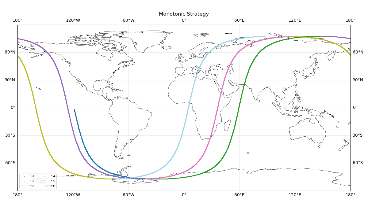
Decomposing with Monotonic Segments#
The "monotonic" strategy splits the track every time the latitude changes
direction. This yields tighter bounding boxes and is well suited for
near-polar orbits.
segments_mono = satellite.decompose_track(
    lon,
    lat,
    strategy="monotonic",
    opts=satellite.DecompositionOptions()
    .with_min_edge_size(1)
    .with_merge_area_ratio(0.0),
)

print(f"\nMonotonic strategy → {len(segments_mono)} segment(s)")
for seg in segments_mono:
    print(f"  {seg}")
Monotonic strategy → 6 segment(s)
  TrackSegment([0, 4899], zone=mid, orbit=prograde, bbox=lon[-118.71,-29.48] lat[-77.50,-1.72])
  TrackSegment([4899, 14857], zone=mid, orbit=prograde, bbox=lon[-29.48,146.75] lat[-77.50,77.73])
  TrackSegment([14857, 24703], zone=mid, orbit=prograde, bbox=lon[-179.98,179.96] lat[-77.36,77.73])
  TrackSegment([24703, 34509], zone=mid, orbit=prograde, bbox=lon[-46.32,117.38] lat[-77.36,77.39])
  TrackSegment([34509, 44328], zone=mid, orbit=prograde, bbox=lon[-179.99,180.00] lat[-77.44,77.39])
  TrackSegment([44328, 54157], zone=mid, orbit=prograde, bbox=lon[-77.86,87.68] lat[-77.44,77.48])
Custom Options with the Builder Pattern#
DecompositionOptions is configured
with a fluent builder. Here we restrict the polar zones to ±70° and expand
each segment’s bounding box by a 250 km swath width.
opts = (
    satellite.DecompositionOptions()
    .with_south_limit(-70.0)
    .with_north_limit(70.0)
    .with_swath_width_km(250.0)
)

segments_custom = satellite.decompose_track(
    lon, lat, strategy="latitude_bands", opts=opts
)

print(f"\nCustom options → {len(segments_custom)} segment(s)")
for seg in segments_custom:
    print(
        f"  indices [{seg.first_index}:{seg.last_index}]  "
        f"zone={seg.zone.name:<6}  orbit={seg.orbit.name}  "
        f"size={seg.size}  bbox={seg.bbox}"
    )
Custom options → 12 segment(s)
  indices [0:4025]  zone=MID     orbit=PROGRADE  size=4026  bbox=[(-122.18035730711759, -71.11497126867037) to (-78.28394910768316, -0.5950752897835188)]
  indices [4026:5769]  zone=SOUTH   orbit=PROGRADE  size=1744  bbox=[(-87.42217801429898, -78.62207458938778) to (28.22878765387446, -68.88060095315412)]
  indices [5770:13994]  zone=MID     orbit=PROGRADE  size=8225  bbox=[(19.089670274396653, -71.11756095998514) to (98.8763230766995, 71.11856670388329)]
  indices [13995:15718]  zone=NORTH   orbit=PROGRADE  size=1724  bbox=[(-185.79262505284677, 68.88443632406745) to (185.7785311803342, 78.85227574922901)]
  indices [15719:23935]  zone=MID     orbit=PROGRADE  size=8217  bbox=[(-165.454652420263, -71.12051016104613) to (-86.36475207056257, 71.12012502888109)]
  indices [23936:25498]  zone=SOUTH   orbit=PROGRADE  size=1563  bbox=[(-95.4372713588437, -78.48356264128525) to (5.12997545291418, -68.88495302270005)]
  indices [25499:33729]  zone=MID     orbit=PROGRADE  size=8231  bbox=[(-3.9424307199328825, -71.11919721464518) to (76.33448543737813, 71.1226005345747)]
  indices [33730:35300]  zone=NORTH   orbit=PROGRADE  size=1571  bbox=[(67.24812324802451, 68.88409658157624) to (168.5006594631517, 78.51219016387282)]
  indices [35301:43532]  zone=MID     orbit=PROGRADE  size=8232  bbox=[(-183.46150752788915, -71.11659757023207) to (183.47303810989328, 71.11834021263454)]
  indices [43533:45123]  zone=SOUTH   orbit=PROGRADE  size=1591  bbox=[(-129.30989934815491, -78.56274179493369) to (-26.391986201746143, -68.88236754620849)]
  indices [45124:53354]  zone=MID     orbit=PROGRADE  size=8231  bbox=[(-35.503151452778376, -71.12402615281087) to (44.768934811200566, 71.11923375754627)]
  indices [53355:54157]  zone=NORTH   orbit=PROGRADE  size=803  bbox=[(35.63593216616117, 68.88501343221873) to (93.36703444585453, 78.60714213805568)]
Accessing Individual Segments#
Each TrackSegment exposes the index
range so you can slice the original arrays directly.
print("\nSlicing the track for each segment (latitude_bands):")
for seg in segments_bands:
    sl = slice(seg.first_index, seg.last_index + 1)
    lon_seg = lon[sl]
    lat_seg = lat[sl]
    print(
        f"  zone={seg.zone.name:<6}  orbit={seg.orbit.name:<11}  "
        f"points={seg.size:4d}  "
        f"lat=[{lat_seg.min():+.1f}°, {lat_seg.max():+.1f}°]"
    )
Slicing the track for each segment (latitude_bands):
  zone=MID     orbit=PROGRADE     points=2772  lat=[-50.0°, -1.7°]
  zone=SOUTH   orbit=PROGRADE     points=4248  lat=[-77.5°, -50.0°]
  zone=MID     orbit=PROGRADE     points=5729  lat=[-50.0°, +50.0°]
  zone=NORTH   orbit=PROGRADE     points=4215  lat=[+50.0°, +77.7°]
  zone=MID     orbit=PROGRADE     points=5727  lat=[-50.0°, +50.0°]
  zone=SOUTH   orbit=PROGRADE     points=4058  lat=[-77.4°, -50.0°]
  zone=MID     orbit=PROGRADE     points=5732  lat=[-50.0°, +50.0°]
  zone=NORTH   orbit=PROGRADE     points=4070  lat=[+50.0°, +77.4°]
  zone=MID     orbit=PROGRADE     points=5733  lat=[-50.0°, +50.0°]
  zone=SOUTH   orbit=PROGRADE     points=4090  lat=[-77.4°, -50.0°]
  zone=MID     orbit=PROGRADE     points=5732  lat=[-50.0°, +50.0°]
  zone=NORTH   orbit=PROGRADE     points=2052  lat=[+50.0°, +77.5°]
Visualizing the Segments#
Plot each decomposition strategy separately: - latitude_bands: color by latitude zone (south/mid/north) - monotonic: color by segment index (zone is not the relevant split axis)
zone_colors = {
    satellite.LatitudeZone.SOUTH: "#1f77b4",  # blue
    satellite.LatitudeZone.MID: "#ff7f0e",  # orange
    satellite.LatitudeZone.NORTH: "#2ca02c",  # green
}

# Latitude-bands view: colors reflect dominant latitude zone.
fig = plt.figure(figsize=(12, 7))
ax = plt.axes(projection=ccrs.PlateCarree())
ax.set_global()
ax.coastlines(linewidth=0.5)
ax.gridlines(draw_labels=True, linewidth=0.4, alpha=0.5)
ax.set_title("Latitude Bands Strategy")

for seg in segments_bands:
    sl = slice(seg.first_index, seg.last_index + 1)
    ax.plot(
        lon[sl],
        lat[sl],
        ".",
        color=zone_colors[seg.zone],
        markersize=2,
        transform=ccrs.Geodetic(),
    )

legend_patches = [
    mpatches.Patch(color=zone_colors[z], label=z.name.capitalize())
    for z in satellite.LatitudeZone
]
ax.legend(handles=legend_patches, loc="lower left", fontsize=8)

plt.tight_layout()

# Monotonic view: colors reflect segment identity, not zone.
fig = plt.figure(figsize=(12, 7))
ax = plt.axes(projection=ccrs.PlateCarree())
ax.set_global()
ax.coastlines(linewidth=0.5)
ax.gridlines(draw_labels=True, linewidth=0.4, alpha=0.5)
ax.set_title("Monotonic Strategy")

segment_colors = plt.cm.tab20(np.linspace(0.0, 1.0, len(segments_mono)))

for index, seg in enumerate(segments_mono, start=1):
    sl = slice(seg.first_index, seg.last_index + 1)
    ax.plot(
        lon[sl],
        lat[sl],
        ".",
        color=segment_colors[index - 1],
        markersize=2,
        transform=ccrs.Geodetic(),
        label=f"S{index}",
    )

ax.legend(loc="lower left", fontsize=8, ncol=2)

plt.tight_layout()
Total running time of the script: (0 minutes 1.533 seconds)