Optimal Interpolation (OI) — global mode (lon, lat, time)

This example illustrates the geographic mode of pyinterp.OptimalInterpolation, which is the appropriate setup for operational altimetry products such as DUACS / AVISO sea-level analyses.

In this mode the wrapper:

• converts the user’s (lon, lat) coordinates to ECEF internally — the R-tree’s k-nearest-neighbour search then uses the geodetic chord distance, which is the right metric on the globe;

• keeps the original (lon, lat) to sample any pyinterp.Grid2D parameter (decorrelation length, field standard deviation) — no inverse projection is needed because the geographic coordinates are preserved end-to-end;

• applies the spatial decorrelation scale l_spatial (in meters) isotropically to the three ECEF axes — appropriate for the standard altimetry assumption of isotropic horizontal covariance.

Compared to the regional / cartesian example, the user no longer needs to pre-project their observations, and the analysis is correct globally (no equatorial cos(lat) distortion, no projection artefacts).

import matplotlib.pyplot as plt
import numpy as np

import pyinterp

Synthetic truth

A slowly evolving SLA-like field on a regional patch of the North Atlantic (we keep the domain small only to make the figure readable; the same code works at planetary scale).

def true_field(lon, lat, t_seconds):
    """Toy SLA: sinusoidal, slowly drifting eastward with time."""
    lon_phase = np.deg2rad(lon) - 1.0e-6 * t_seconds  # ~5 deg / day
    lat_phase = np.deg2rad(lat)
    return 0.2 * np.sin(3.0 * lon_phase) * np.cos(2.0 * lat_phase)

Scattered along-track observations (two missions)

rng = np.random.default_rng(42)
n_obs = 600
lon = rng.uniform(-30.0, 0.0, n_obs)
lat = rng.uniform(30.0, 50.0, n_obs)
t = rng.uniform(0.0, 5 * 86400.0, n_obs)  # 5-day window

mission = rng.integers(0, 2, n_obs)
sigma_per_mission = np.array([0.02, 0.06])  # meters
sigma_obs = sigma_per_mission[mission]
obs_value = true_field(lon, lat, t) + rng.normal(0.0, sigma_obs)
obs_sigma2 = sigma_obs ** 2

Build the geographic OI estimator

In geographic mode the packed coordinates are ECEF metres plus time in seconds, and the k-nearest-neighbour search ranks by their raw Euclidean mix — which is unrelated to how correlated observations actually are. We rescale time to a metres-equivalent with time_scale ≈ L_spatial / L_t (metres per second) so the neighbour search is balanced between space and time. It cancels out of the covariance, so it only affects which neighbours are retrieved. time_scale is fixed at construction, so we pick a single representative value — fine even when L_spatial varies regionally (see the Grid2D section below).

L_SPATIAL = 150e3        # metres
L_TIME = 7 * 86400.0     # seconds (7-day temporal decorrelation)
time_scale = L_SPATIAL / L_TIME  # ≈ 0.25 m/s

oi = pyinterp.OptimalInterpolation(
    np.column_stack([lon, lat, t]),
    obs_value,
    obs_sigma2,
    covariance="gaussian",
    coordinate_system="geographic",
    time_scale=time_scale,
)

Analysis grid

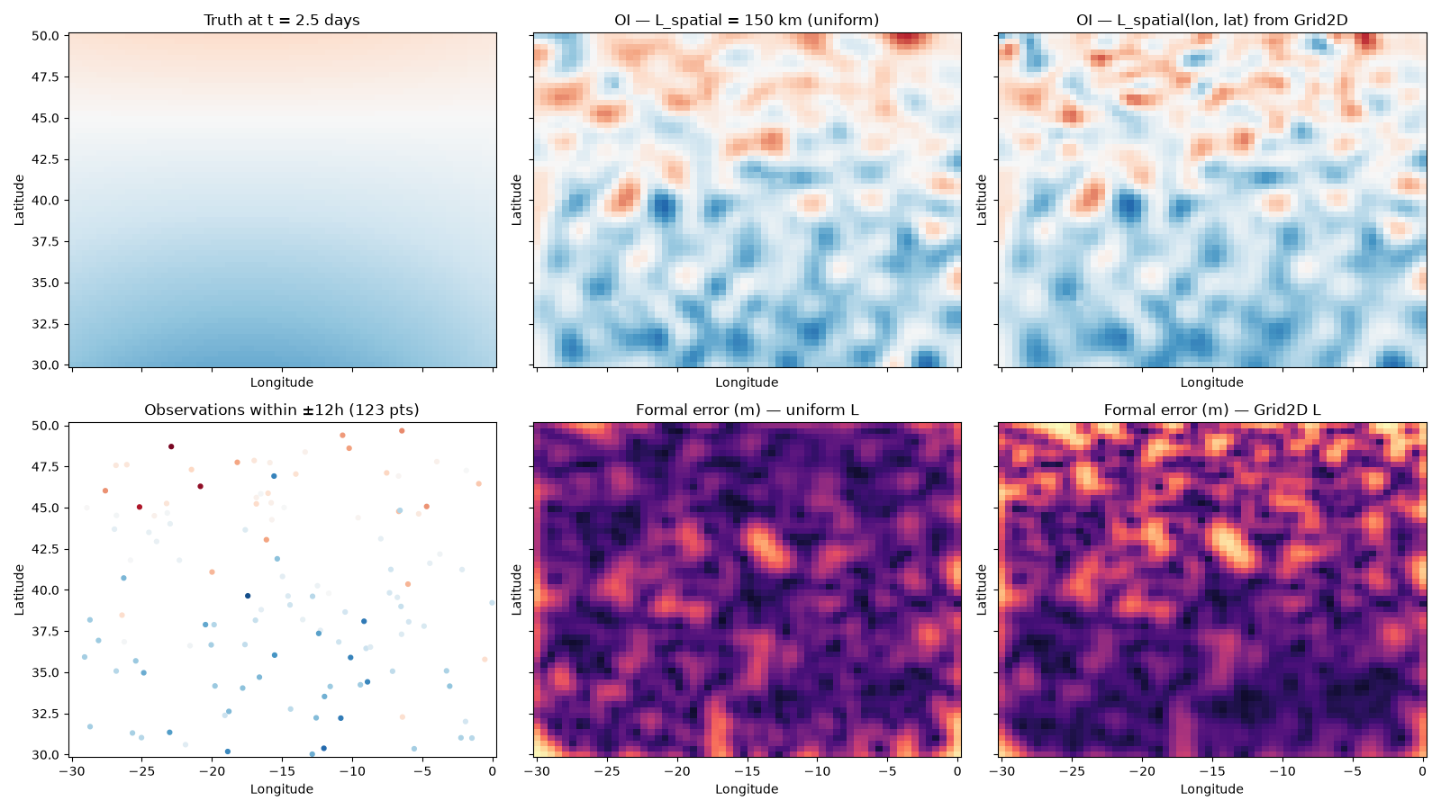
Reconstruct the field at t = 2.5 days on a regular (lon, lat) mesh.

nlon, nlat = 60, 60
glon = np.linspace(-30.0, 0.0, nlon)
glat = np.linspace(30.0, 50.0, nlat)
mlon, mlat = np.meshgrid(glon, glat, indexing="ij")
mt = np.full(mlon.size, 2.5 * 86400.0)
query = np.column_stack([mlon.ravel(), mlat.ravel(), mt])

Uniform spatial scale

150 km horizontal decorrelation, 7-day temporal decorrelation, σ = 20 cm.

res_uniform = oi(
    query,
    l_spatial=L_SPATIAL,    # metres
    lt=L_TIME,              # seconds
    sigma=0.20,             # metres
    k=24,
)
field_uniform = res_uniform.value.reshape(mlon.shape)
error_uniform = res_uniform.error.reshape(mlon.shape)

Spatially-varying decorrelation length (Grid2D)

A coarse climatological grid where decorrelation grows from 80 km in the north (rough seasonal variability) to 200 km in the south (smoother subtropical gyre).

ax_lon = pyinterp.Axis(np.linspace(-30.0, 0.0, 11))
ax_lat = pyinterp.Axis(np.linspace(30.0, 50.0, 11))
ls_grid_array = np.linspace(200e3, 80e3, 11)[None, :] * np.ones((11, 11))
grid_ls = pyinterp.Grid2D(ax_lon, ax_lat, ls_grid_array)

res_varying = oi(
    query,
    l_spatial=grid_ls,
    lt=L_TIME,
    sigma=0.20,
    k=24,
)
field_varying = res_varying.value.reshape(mlon.shape)
error_varying = res_varying.error.reshape(mlon.shape)

Visualisation

truth = true_field(mlon, mlat, 2.5 * 86400.0)

fig, axes = plt.subplots(2, 3, figsize=(16, 9), sharex=True, sharey=True)

axes[0, 0].pcolormesh(mlon, mlat, truth, vmin=-0.2, vmax=0.2, cmap="RdBu_r")
axes[0, 0].set_title("Truth at t = 2.5 days")

axes[0, 1].pcolormesh(
    mlon, mlat, field_uniform, vmin=-0.2, vmax=0.2, cmap="RdBu_r"
)
axes[0, 1].set_title("OI — L_spatial = 150 km (uniform)")

axes[0, 2].pcolormesh(
    mlon, mlat, field_varying, vmin=-0.2, vmax=0.2, cmap="RdBu_r"
)
axes[0, 2].set_title("OI — L_spatial(lon, lat) from Grid2D")

near_t = np.abs(t - 2.5 * 86400.0) < 0.5 * 86400.0
axes[1, 0].scatter(
    lon[near_t], lat[near_t], c=obs_value[near_t],
    vmin=-0.2, vmax=0.2, cmap="RdBu_r", s=12
)
axes[1, 0].set_title(f"Observations within ±12h ({near_t.sum()} pts)")

axes[1, 1].pcolormesh(
    mlon, mlat, error_uniform, vmin=0.0, vmax=0.20, cmap="magma"
)
axes[1, 1].set_title("Formal error (m) — uniform L")

axes[1, 2].pcolormesh(
    mlon, mlat, error_varying, vmin=0.0, vmax=0.20, cmap="magma"
)
axes[1, 2].set_title("Formal error (m) — Grid2D L")

for ax in axes.flat:
    ax.set_xlabel("Longitude")
    ax.set_ylabel("Latitude")

fig.tight_layout()
plt.show()