Optimal Interpolation (OI) — 2D + time

This example illustrates how to reconstruct a 2D field that evolves in time from scattered observations using pyinterp.OptimalInterpolation.

The OI estimator is the BLUE (Best Linear Unbiased Estimator) commonly used in operational altimetry to map sea-level anomalies (SLA) from satellite along-track data. Two features make OptimalInterpolation well suited for this:

• an anisotropic Gaussian-family covariance kernel — the decorrelation scales in space (Lx, Ly) and time (Lt) are specified independently;

• a per-observation error variance σ²_obs, so that observations from different sources (missions, instruments) can be weighted by their own noise level.

Both Lx, Ly, Lt and the field standard deviation σ may be either scalars or pyinterp.Grid2D objects, which lets you tune the analysis regionally — for instance, increasing Lx/Ly over the open ocean and shrinking them in coastal regions.

import matplotlib.pyplot as plt
import numpy as np

import pyinterp

Synthetic truth

We build an evolving 2D field on a small domain. This is the “truth” we will try to recover from sparse, noisy samples.

def true_field(x, y, t):
    """A slowly evolving 2D field used as the analysis target."""
    return (
        np.sin(0.5 * x + 0.1 * t)
        * np.cos(0.4 * y - 0.05 * t)
    )

Sparse observations

We sample the field at random (x, y, t) locations. To mimic a multi-mission setting we assign two different noise levels (e.g. an accurate mission and a noisier one).

rng = np.random.default_rng(42)
n_obs = 400
obs_x = rng.uniform(0.0, 10.0, n_obs)
obs_y = rng.uniform(0.0, 10.0, n_obs)
obs_t = rng.uniform(0.0, 5.0, n_obs)
mission = rng.integers(0, 2, n_obs)  # 0 or 1
sigma_per_mission = np.array([0.05, 0.15])
sigma_obs = sigma_per_mission[mission]
obs_value = true_field(obs_x, obs_y, obs_t) + rng.normal(0.0, sigma_obs)
obs_sigma2 = sigma_obs ** 2

Building the OI estimator

The k-nearest-neighbour search ranks observations by Euclidean distance in the packed (x, y, t) space, which mixes spatial units with time. time_scale rescales the time axis so that a one-decorrelation-length step in space and one in time map to the same packed distance; the k retrieved neighbours are then the k most correlated observations rather than merely the spatially closest ones. The rule of thumb is time_scale ≈ L_spatial / L_t. It cancels out of the covariance, so it only changes neighbour selection — never the analysis when k = N.

We derive time_scale from the decorrelation scales we will analyse with (set here so the example stays self-consistent):

L_SPACE = 1.5  # decorrelation length in x and y
L_TIME = 1.0   # decorrelation length in t
time_scale = L_SPACE / L_TIME

oi = pyinterp.OptimalInterpolation(
    np.column_stack([obs_x, obs_y, obs_t]),
    obs_value,
    obs_sigma2,
    covariance="gaussian",
    time_scale=time_scale,
)

Analysis grid

We reconstruct the field at t = 2.5 (mid-window) on a regular 2D grid.

nx, ny = 60, 60
ax_x = np.linspace(0.0, 10.0, nx)
ax_y = np.linspace(0.0, 10.0, ny)
xx, yy = np.meshgrid(ax_x, ax_y, indexing="ij")
tt = np.full(xx.size, 2.5)
query = np.column_stack([xx.ravel(), yy.ravel(), tt])

Constant length scales

We first run the OI with uniform length scales.

result_uniform = oi(
    query,
    lx=L_SPACE,
    ly=L_SPACE,
    lt=L_TIME,
    sigma=1.0,
    k=24,
    num_threads=0,
)
field_uniform = result_uniform.value.reshape(xx.shape)
error_uniform = result_uniform.error.reshape(xx.shape)

Spatially-varying length scales

Real operational products tune Lx, Ly, Lt and σ regionally. We build small Grid2D objects to demonstrate this: shorter decorrelation in the left half of the domain, longer on the right.

gx_axis = pyinterp.Axis(np.linspace(0.0, 10.0, 11))
gy_axis = pyinterp.Axis(np.linspace(0.0, 10.0, 11))
lx_grid_array = np.linspace(0.6, 2.4, 11)[:, None] * np.ones((11, 11))
ly_grid_array = lx_grid_array
lx_grid = pyinterp.Grid2D(gx_axis, gy_axis, lx_grid_array)
ly_grid = pyinterp.Grid2D(gx_axis, gy_axis, ly_grid_array)

result_varying = oi(
    query,
    lx=lx_grid,
    ly=ly_grid,
    lt=L_TIME,
    sigma=1.0,
    k=24,
)
field_varying = result_varying.value.reshape(xx.shape)
error_varying = result_varying.error.reshape(xx.shape)

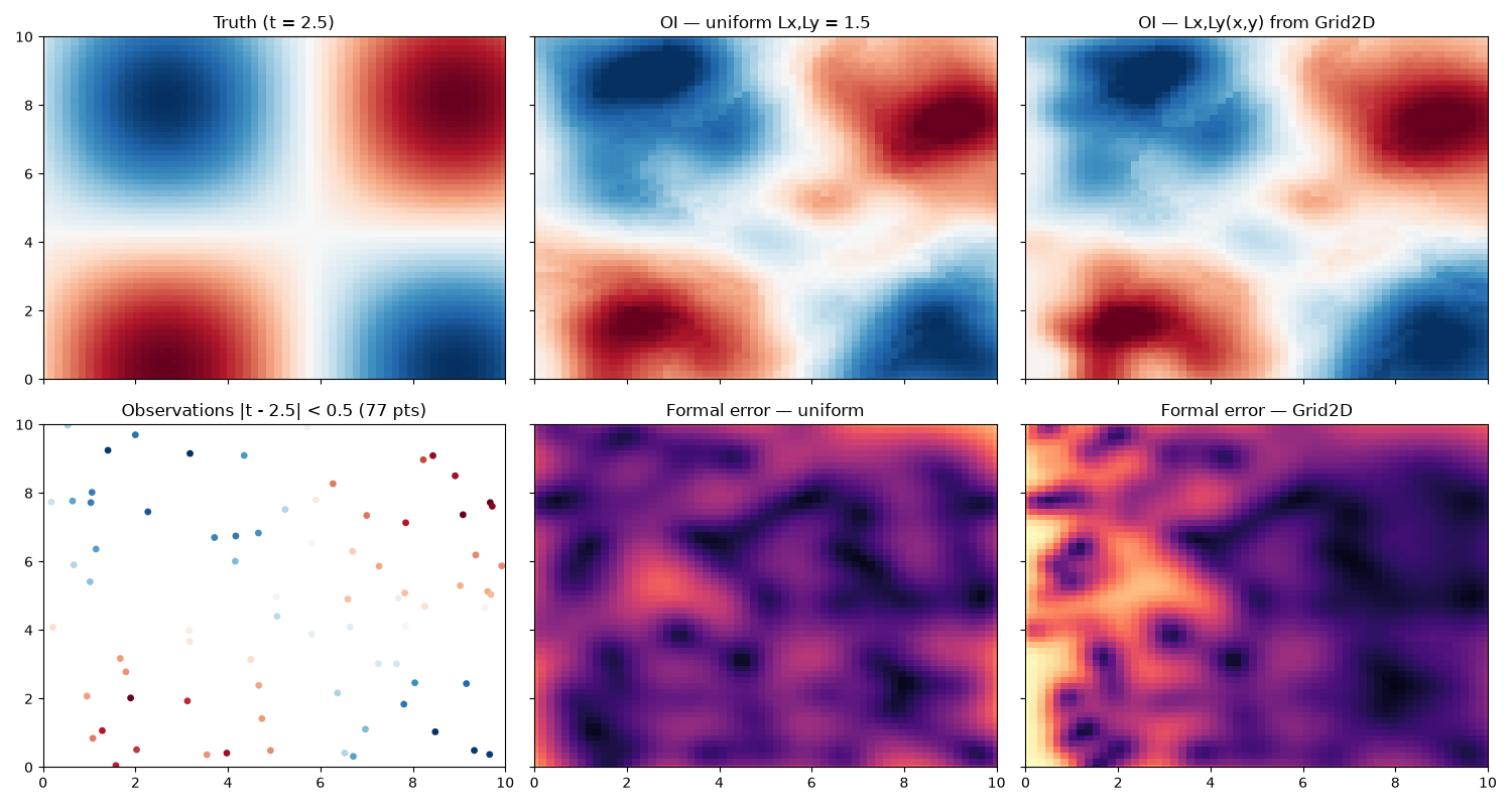
Visualisation

truth = true_field(xx, yy, 2.5)

fig, axes = plt.subplots(2, 3, figsize=(15, 8), sharex=True, sharey=True)

axes[0, 0].pcolormesh(xx, yy, truth, vmin=-1, vmax=1, cmap="RdBu_r")
axes[0, 0].set_title("Truth (t = 2.5)")

axes[0, 1].pcolormesh(xx, yy, field_uniform, vmin=-1, vmax=1, cmap="RdBu_r")
axes[0, 1].set_title("OI — uniform Lx,Ly = 1.5")

axes[0, 2].pcolormesh(xx, yy, field_varying, vmin=-1, vmax=1, cmap="RdBu_r")
axes[0, 2].set_title("OI — Lx,Ly(x,y) from Grid2D")

# Bottom row: errors and observation locations
near_t = np.abs(obs_t - 2.5) < 0.5
axes[1, 0].scatter(
    obs_x[near_t], obs_y[near_t], c=obs_value[near_t],
    vmin=-1, vmax=1, cmap="RdBu_r", s=15
)
axes[1, 0].set_title(f"Observations |t - 2.5| < 0.5 ({near_t.sum()} pts)")

axes[1, 1].pcolormesh(xx, yy, error_uniform, vmin=0, vmax=1, cmap="magma")
axes[1, 1].set_title("Formal error — uniform")

axes[1, 2].pcolormesh(xx, yy, error_varying, vmin=0, vmax=1, cmap="magma")
axes[1, 2].set_title("Formal error — Grid2D")

for ax in axes.flat:
    ax.set_xlim(0, 10)
    ax.set_ylim(0, 10)

fig.tight_layout()
plt.show()