Geodesic Distances in RTree3D

pyinterp.RTree3D() indexes scattered points and finds their nearest neighbours. The way it measures distances depends on how it is built: as plain Cartesian coordinates, as straight-line (chord) distances in Earth-centred coordinates, or as geodesic distances on the ellipsoid. In this example, you will learn how the three modes differ, when they find different neighbours, and how this affects an inverse distance weighting interpolation.

import pickle
import time

import matplotlib.pyplot
import numpy

import pyinterp
from pyinterp.geometry import geographic

Scattered Observations

We draw 400 stations uniformly distributed on the sphere: a sparse network, so the neighbours of a point are hundreds or thousands of kilometres away. Each station measures a smooth synthetic field.

rng = numpy.random.default_rng(0)
lon = rng.uniform(-180.0, 180.0, 400)
lat = numpy.degrees(numpy.arcsin(rng.uniform(-1.0, 1.0, 400)))
coordinates = numpy.column_stack((lon, lat))


def field(lon, lat):
    """Synthetic field sampled by the stations."""
    return numpy.cos(numpy.radians(lat)) ** 2 * numpy.sin(
        3.0 * numpy.radians(lon)
    ) + numpy.sin(numpy.radians(lat))


values = field(lon, lat)

Building the Trees

We build the three kinds of pyinterp.RTree3D():

• without a spheroid (the default), the longitudes and latitudes are taken as Cartesian x and y, and distances are expressed in degrees;

• with a spheroid, the points are converted to ECEF coordinates and ranked by their straight-line (chord) distance, in metres;

• with distance="geodesic", the tree still searches in ECEF, but ranks the neighbours by their geodesic distance on the spheroid.

We also build a pyinterp.geometry.geographic.RTree, which uses geodesic distances on WGS-84 throughout. packing loads all the points at once, which builds a better balanced tree than repeated insert calls.

wgs84 = geographic.Spheroid()
trees = {
    "cartesian": pyinterp.RTree3D(),
    "chord": pyinterp.RTree3D(wgs84),
    "geodesic": pyinterp.RTree3D(wgs84, distance="geodesic"),
    "geographic": geographic.RTree(),
}
for tree in trees.values():
    tree.packing(coordinates, values)
print(trees["geodesic"].distance, trees["geodesic"].size())

geodesic 400

The tree keeps its spheroid and distance mode when it is pickled.

print(pickle.loads(pickle.dumps(trees["geodesic"])).distance)

geodesic

Querying the Nearest Neighbours

pyinterp.rtree.query() returns, for each query point, the distances to its k nearest neighbours and their values. We query a point on the equator, one next to the antimeridian and one close to the North Pole.

targets = numpy.array([[0.0, 0.0], [179.0, 10.0], [20.0, 85.0]])
neighbours = {
    name: pyinterp.rtree.query(tree, targets, k=4)
    for name, tree in trees.items()
}
for name, (distance, _) in neighbours.items():
    print(f"{name:>10}:", numpy.array2string(distance[:, 0], precision=1))

 cartesian: [ 6.6  2.9 11.3]
     chord: [736756.9 323544.4 283147.5]
  geodesic: [737162.  323576.5 283167.5]
geographic: [737162.  323576.5 283167.5]

The Cartesian tree measures distances in degrees on a flat map: it does not know that longitude 179° is next to -179°, nor that the meridians converge at the poles. Next to the antimeridian and the pole, it returns other stations than the geodesic search (compare the values found):

for name in ("cartesian", "chord"):
    same = numpy.isin(neighbours[name][1], neighbours["geodesic"][1])
    print(f"{name:>10}: common neighbours per point", same.sum(axis=1))

cartesian: common neighbours per point [4 3 1]
    chord: common neighbours per point [4 4 4]

The chord and geodesic trees find the same stations. The geographic RTree returns exactly the same distances as the geodesic RTree3D():

print(numpy.allclose(neighbours["geodesic"][0], neighbours["geographic"][0]))

True

Chord versus Geodesic Distances

A chord cuts through the Earth, so it is always shorter than the geodesic. The gap is negligible at short range but grows with the distance. We query the 32 nearest stations of random points and compare both distances.

points = numpy.column_stack(
    (
        rng.uniform(-180.0, 180.0, 2000),
        numpy.degrees(numpy.arcsin(rng.uniform(-1.0, 1.0, 2000))),
    )
)
chord, chord_values = pyinterp.rtree.query(trees["chord"], points, k=32)
geodesic, geodesic_values = pyinterp.rtree.query(
    trees["geodesic"], points, k=32
)
# Both trees return the neighbours sorted by their own distance: matching them
# by rank only works where the order agrees.
same_order = numpy.all(chord_values == geodesic_values, axis=1)
print(f"Same ranking of the 32 neighbours: {same_order.mean():.1%} of points")

fig, ax = matplotlib.pyplot.subplots(figsize=(8, 4.5), layout="constrained")
ax.scatter(
    geodesic[same_order].ravel() * 1e-3,
    100.0 * (1.0 - chord[same_order].ravel() / geodesic[same_order].ravel()),
    s=2,
    color="tab:blue",
    alpha=0.3,
)
ax.set_xlabel("Geodesic distance (km)")
ax.set_ylabel("Chord shortfall (%)")
ax.set_title("How much shorter the chord is than the geodesic")
ax.grid(True, alpha=0.3)

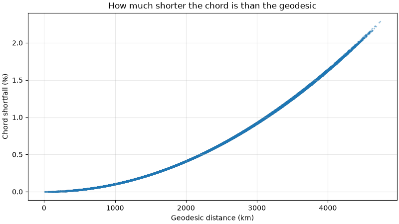
Same ranking of the 32 neighbours: 97.7% of points

Where the ranking differs, two stations are almost at the same distance: the shortfall of the chord grows with the distance and, on an ellipsoid, also depends on the direction, which is enough to swap them.

Inverse Distance Weighting

We now interpolate the stations on a global 1° grid with pyinterp.rtree.inverse_distance_weighting(), using the 8 nearest neighbours, and compare each mode with the geodesic one.

mx, my = numpy.meshgrid(
    numpy.arange(-179.5, 180.0, 1.0),
    numpy.arange(-89.5, 90.0, 1.0),
)
grid = numpy.column_stack((mx.ravel(), my.ravel()))
idw = {}
for name, tree in trees.items():
    result, _ = pyinterp.rtree.inverse_distance_weighting(tree, grid, k=8, p=2)
    idw[name] = result.reshape(mx.shape)

fig, axes = matplotlib.pyplot.subplots(
    1, 2, figsize=(10, 4.5), layout="constrained", sharey=True
)
for ax, name, vmax in zip(
    axes, ("cartesian", "chord"), (0.3, 0.001), strict=True
):
    image = ax.pcolormesh(
        mx,
        my,
        idw[name] - idw["geodesic"],
        cmap="RdBu_r",
        vmin=-vmax,
        vmax=vmax,
        shading="auto",
    )
    ax.scatter(lon, lat, s=2, color="black")
    ax.set_title(f"{name} - geodesic")
    ax.set_xlabel("Longitude (°)")
    fig.colorbar(
        image,
        ax=ax,
        orientation="horizontal",
        shrink=0.8,
        ticks=numpy.linspace(-vmax, vmax, 5),
    )
axes[0].set_ylabel("Latitude (°)")
for name in ("cartesian", "chord", "geographic"):
    error = numpy.abs(idw[name] - idw["geodesic"]).max()
    print(f"{name:>10}: max |difference| = {error:.3g}")

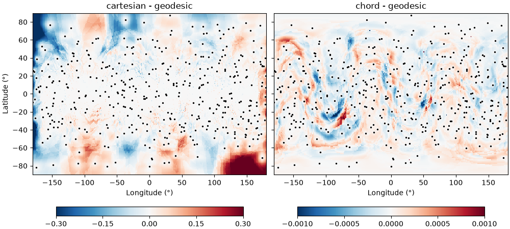
 cartesian: max |difference| = 0.598
     chord: max |difference| = 0.0494
geographic: max |difference| = 2.73e-15

The Cartesian interpolation is wrong at high latitudes and along the antimeridian, where it picks the wrong neighbours. The chord interpolation differs by less than 0.001 almost everywhere (note the colour scales): since the chord shortens long distances more than short ones, its weights favour the farthest neighbours a little more. Its maximum difference comes from the rare points where a near-tie swaps the eighth neighbour. The geographic and geodesic trees give the same field.

Query Speed

The geodesic RTree3D() searches its nodes with fast ECEF distances and computes geodesics only to rank the candidates, while the geographic tree evaluates geodesics everywhere.

for name, tree in trees.items():
    start = time.perf_counter()
    pyinterp.rtree.query(tree, grid, k=8)
    print(f"{name:>10}: {1e3 * (time.perf_counter() - start):6.1f} ms")

 cartesian:   31.1 ms
     chord:   28.8 ms
  geodesic:  153.2 ms
geographic: 1164.3 ms