Basic Geometric Primitives

This example demonstrates the fundamental geometric objects available in the pyinterp.geometry module. These primitives form the building blocks for spatial operations in both geographic (lon/lat on a spheroid) and cartesian (x/y plane) coordinate systems.

The geometry module provides a comprehensive set of primitives that mirror standard GIS formats like WKT and GeoJSON, making it easy to work with spatial data from various sources.

Primitives Covered:

Class	Description
Spheroid	Reference ellipsoid
Point	Single location
Segment	Line between two points
Box	Rectangular area
LineString	Sequence of points
Ring	Closed boundary
Polygon	Area with optional holes
MultiPoint	Point collection
MultiLineString	LineString collection
MultiPolygon	Polygon collection

Let’s start by importing the necessary libraries.

import json

import cartopy.crs
import cartopy.feature
import matplotlib.pyplot
import numpy
from pyinterp.geometry import cartesian, geographic

Spheroid: Reference Ellipsoid

The Spheroid class represents the reference ellipsoid used for geodetic calculations. By default, it uses WGS84.

wgs84 = geographic.Spheroid()
print("WGS84 Properties:")
print(f"  Semi-major axis: {wgs84.semi_major_axis:,.2f} m")
print(f"  Flattening: {wgs84.flattening:.10f}")
print(f"  Mean radius: {wgs84.mean_radius():,.2f} m")
print(f"  Authalic radius: {wgs84.authalic_radius():,.2f} m")
print(f"  Equatorial circumference: {wgs84.equatorial_circumference():,.2f} m")

WGS84 Properties:
  Semi-major axis: 6,378,137.00 m
  Flattening: 0.0033528107
  Mean radius: 6,371,008.77 m
  Authalic radius: 6,371,007.18 m
  Equatorial circumference: 40,075,016.69 m

You can define custom ellipsoids by providing the semi-major axis and flattening.

grs80 = geographic.Spheroid(6378137.0, 1 / 298.257222101)
difference = abs(wgs84.semi_major_axis - grs80.semi_major_axis)
print("\nGRS80 Properties:")
print(f"  Semi-major axis: {grs80.semi_major_axis:,.2f} m")
print(f"  Flattening: {grs80.flattening:.10f}")
print(f"  Difference from WGS84: {difference:.6f} m")

GRS80 Properties:
  Semi-major axis: 6,378,137.00 m
  Flattening: 0.0033528107
  Difference from WGS84: 0.000000 m

Point: Single Geographic Location

A Point represents a single location defined by longitude and latitude in degrees.

paris = geographic.Point(2.3488, 48.8534)
new_york = geographic.Point(-73.9385, 40.6643)
london = geographic.Point(-0.1276, 51.5074)
tokyo = geographic.Point(139.6917, 35.6895)

print("\nGeographic Points:")
print(f"  Paris: {paris}")
print(f"  New York: {new_york}")
print(f"  London: {london}")
print(f"  Tokyo: {tokyo}")

Geographic Points:
  Paris: (2.3488, 48.8534)
  New York: (-73.9385, 40.6643)
  London: (-0.1276, 51.5074)
  Tokyo: (139.6917, 35.6895)

Points support equality comparison and hashing

print(f"\nParis == Paris: {paris == paris}")  # noqa: PLR0124
print(f"Paris == London: {paris == london}")
print(f"Hash of Paris: {hash(paris)}")

Paris == Paris: True
Paris == London: False
Hash of Paris: 1223149219523137366

Segment: Line Between Two Points

A Segment represents a straight line between two points.

segment = geographic.Segment((paris.lon, paris.lat), (london.lon, london.lat))
print("\nSegment:")
print(f"  Start: ({segment.a.lon:.4f}, {segment.a.lat:.4f})")
print(f"  End: ({segment.b.lon:.4f}, {segment.b.lat:.4f})")
print(f"  Length: {len(segment)} points")

# Segments are iterable
for i, point in enumerate(segment):
    print(f"  Point {i}: ({point.lon:.4f}, {point.lat:.4f})")

Segment:
  Start: (2.3488, 48.8534)
  End: (-0.1276, 51.5074)
  Length: 2 points
  Point 0: (2.3488, 48.8534)
  Point 1: (-0.1276, 51.5074)

Box: Rectangular Geographic Area

A Box defines a rectangular area from two corner points.

box = geographic.Box((new_york.lon, new_york.lat), (paris.lon, paris.lat))
print("\nBox:")
print(f"  Min corner: ({box.min_corner.lon:.4f}, {box.min_corner.lat:.4f})")
print(f"  Max corner: ({box.max_corner.lon:.4f}, {box.max_corner.lat:.4f})")

# Get the centroid of the box
centroid = geographic.algorithms.centroid(box)
print(f"  Centroid: ({centroid.lon:.4f}, {centroid.lat:.4f})")

Box:
  Min corner: (-73.9385, 40.6643)
  Max corner: (2.3488, 48.8534)
  Centroid: (-35.7949, 44.7588)

Get the envelope (bounding box) of any geometry

envelope = geographic.algorithms.envelope(box)
print(
    f"  Envelope: "
    f"({envelope.min_corner.lon:.4f}, {envelope.min_corner.lat:.4f}) to "
    f"({envelope.max_corner.lon:.4f}, {envelope.max_corner.lat:.4f})"
)

Envelope: (-73.9385, 40.6643) to (2.3488, 48.8534)

LineString: Sequence of Connected Points

A LineString represents a sequence of connected points forming a path.

lon_array = numpy.array([0.0, 1.0, 2.0, 3.0, 4.0], dtype=numpy.float64)
lat_array = numpy.array([0.0, 1.0, 0.5, 1.5, 1.0], dtype=numpy.float64)
line = geographic.LineString(lon_array, lat_array)

print("\nLineString:")
print(f"  Number of points: {len(line)}")
print(f"  Number of segments: {geographic.algorithms.num_segments(line)}")

# LineStrings are iterable
print("  Points:")
for i, point in enumerate(line):
    print(f"    {i}: ({point.lon:.2f}, {point.lat:.2f})")

LineString:
  Number of points: 5
  Number of segments: 4
  Points:
    0: (0.00, 0.00)
    1: (1.00, 1.00)
    2: (2.00, 0.50)
    3: (3.00, 1.50)
    4: (4.00, 1.00)

You can also create an empty LineString and append points

empty_line = geographic.LineString()
empty_line.append(geographic.Point(5.0, 5.0))
empty_line.append(geographic.Point(6.0, 6.0))
print(f"\nLineString created by appending: {len(empty_line)} points")

LineString created by appending: 2 points

Calculate geometric properties

line_length = geographic.algorithms.length(line, spheroid=wgs84)
print(f"\nLineString length: {line_length * 1e-3:.3f} km")

LineString length: 562.338 km

Ring: Closed Boundary

A Ring is a closed linestring that forms a boundary. The first and last points must be identical.

ring_lon = numpy.array([0.0, 4.0, 4.0, 0.0, 0.0], dtype=numpy.float64)
ring_lat = numpy.array([0.0, 0.0, 3.0, 3.0, 0.0], dtype=numpy.float64)
ring = geographic.Ring(ring_lon, ring_lat)

print("\nRing:")
print(f"  Number of points: {len(ring)}")
print(f"  Is closed: {ring[0] == ring[-1]}")

Ring:
  Number of points: 5
  Is closed: True

Polygon: Closed Geographic Shape

A Polygon represents a closed area defined by an outer ring and optional inner rings (holes).

# Simple polygon without holes
outer_lon = numpy.array([0.0, 0.0, 5.0, 5.0, 0.0], dtype=numpy.float64)
outer_lat = numpy.array([0.0, 5.0, 5.0, 0.0, 0.0], dtype=numpy.float64)
outer_ring = geographic.Ring(outer_lon, outer_lat)
polygon = geographic.Polygon(outer_ring)

print("\nSimple Polygon:")
print(f"  Number of points: {geographic.algorithms.num_points(polygon)}")
print(
    f"  Number of interior rings: "
    f"{geographic.algorithms.num_interior_rings(polygon)}"
)

# Calculate area and perimeter
poly_area = geographic.algorithms.area(polygon, spheroid=wgs84)
poly_perimeter = geographic.algorithms.perimeter(polygon, spheroid=wgs84)
print(f"  Area: {poly_area * 1e-6:.2f} km²")
print(f"  Perimeter: {poly_perimeter * 1e-3:.3f} km")

Simple Polygon:
  Number of points: 5
  Number of interior rings: 0
  Area: 307541.81 km²
  Perimeter: 2216.848 km

Polygon with Holes

Create a polygon with an interior hole

# Outer boundary
outer_lon = numpy.array([0.0, 0.0, 10.0, 10.0, 0.0], dtype=numpy.float64)
outer_lat = numpy.array([0.0, 10.0, 10.0, 0.0, 0.0], dtype=numpy.float64)
outer = geographic.Ring(outer_lon, outer_lat)

# Interior hole
hole_lon = numpy.array([3.0, 3.0, 7.0, 7.0, 3.0], dtype=numpy.float64)
hole_lat = numpy.array([3.0, 7.0, 7.0, 3.0, 3.0], dtype=numpy.float64)
hole = geographic.Ring(hole_lon, hole_lat)

# Create polygon with hole
polygon_with_hole = geographic.Polygon(outer, [hole])
num_interior_rings = geographic.algorithms.num_interior_rings(
    polygon_with_hole
)
print("\nPolygon with Hole:")
print(f"  Number of interior rings: {num_interior_rings}")

area_with_hole = geographic.algorithms.area(polygon_with_hole, spheroid=wgs84)
area_outer = geographic.algorithms.area(
    geographic.Polygon(outer), spheroid=wgs84
)
area_hole = geographic.algorithms.area(
    geographic.Polygon(hole), spheroid=wgs84
)
difference = abs((area_outer - area_hole) - area_with_hole)
print(f"  Outer area: {area_outer * 1e-6:.2f} km²")
print(f"  Hole area: {area_hole * 1e-6:.2f} km²")
print(f"  Effective area: {area_with_hole * 1e-6:.2f} km²")
print(
    f"  Expected area: {(area_outer - area_hole) * 1e-6:.2f} km² "
    f"(difference: {difference * 1e-6:.6f} km²)"
)

Polygon with Hole:
  Number of interior rings: 1
  Outer area: 1227877.09 km²
  Hole area: 196255.19 km²
  Effective area: 1424132.29 km²
  Expected area: 1031621.90 km² (difference: 392510.388332 km²)

MultiPoint: Collection of Points

MultiPoint represents a collection of geographic points.

# Create from arrays
lons = numpy.array(
    [paris.lon, new_york.lon, london.lon, tokyo.lon], dtype=numpy.float64
)
lats = numpy.array(
    [paris.lat, new_york.lat, london.lat, tokyo.lat], dtype=numpy.float64
)
cities = geographic.MultiPoint(lons, lats)
num_geometries = geographic.algorithms.num_geometries(cities)
print("\nMultiPoint:")
print(f"  Number of points: {len(cities)}")
print(f"  Number of geometries: {num_geometries}")

# MultiPoints are iterable
print("  Cities:")
for i, city in enumerate(cities):
    print(f"    {i}: ({city.lon:.4f}, {city.lat:.4f})")

MultiPoint:
  Number of points: 4
  Number of geometries: 4
  Cities:
    0: (2.3488, 48.8534)
    1: (-73.9385, 40.6643)
    2: (-0.1276, 51.5074)
    3: (139.6917, 35.6895)

You can also create from a list of Point objects

point_list = [paris, london, tokyo]
cities_from_list = geographic.MultiPoint(point_list)
print(f"\nMultiPoint from list: {len(cities_from_list)} points")

MultiPoint from list: 3 points

MultiLineString: Collection of LineStrings

MultiLineString represents a collection of linestrings.

line1 = geographic.LineString(
    numpy.array([0.0, 1.0, 2.0], dtype=numpy.float64),
    numpy.array([0.0, 1.0, 2.0], dtype=numpy.float64),
)
line2 = geographic.LineString(
    numpy.array([3.0, 4.0, 5.0], dtype=numpy.float64),
    numpy.array([3.0, 4.0, 5.0], dtype=numpy.float64),
)
line3 = geographic.LineString(
    numpy.array([1.0, 2.0, 3.0], dtype=numpy.float64),
    numpy.array([3.0, 2.0, 1.0], dtype=numpy.float64),
)

multiline = geographic.MultiLineString([line1, line2, line3])
num_geometries = geographic.algorithms.num_geometries(multiline)
print("\nMultiLineString:")
print(f"  Number of lines: {len(multiline)}")
print(f"  Number of geometries: {num_geometries}")

# MultiLineStrings are iterable
total_length = 0.0
for i, line in enumerate(multiline):
    length = geographic.algorithms.length(line, spheroid=wgs84)
    total_length += length
    print(f"  Line {i}: {len(line)} points, {length * 1e-3:.3f} km")

print(f"  Total length: {total_length * 1e-3:.3f} km")

MultiLineString:
  Number of lines: 3
  Number of geometries: 3
  Line 0: 3 points, 313.772 km
  Line 1: 3 points, 313.421 km
  Line 2: 3 points, 313.702 km
  Total length: 940.895 km

MultiPolygon: Collection of Polygons

MultiPolygon represents a collection of polygons.

poly1_lon = numpy.array([0.0, 0.0, 3.0, 3.0, 0.0], dtype=numpy.float64)
poly1_lat = numpy.array([0.0, 3.0, 3.0, 0.0, 0.0], dtype=numpy.float64)
poly1 = geographic.Polygon(geographic.Ring(poly1_lon, poly1_lat))

poly2_lon = numpy.array([5.0, 5.0, 8.0, 8.0, 5.0], dtype=numpy.float64)
poly2_lat = numpy.array([5.0, 8.0, 8.0, 5.0, 5.0], dtype=numpy.float64)
poly2 = geographic.Polygon(geographic.Ring(poly2_lon, poly2_lat))

poly3_lon = numpy.array([10.0, 10.0, 12.0, 12.0, 10.0], dtype=numpy.float64)
poly3_lat = numpy.array([0.0, 2.0, 2.0, 0.0, 0.0], dtype=numpy.float64)
poly3 = geographic.Polygon(geographic.Ring(poly3_lon, poly3_lat))

multipoly = geographic.MultiPolygon([poly1, poly2, poly3])
num_geometries = geographic.algorithms.num_geometries(multipoly)
print("\nMultiPolygon:")
print(f"  Number of polygons: {len(multipoly)}")
print(f"  Number of geometries: {num_geometries}")

# MultiPolygons are iterable
total_area = 0.0
for i, poly in enumerate(multipoly):
    area = geographic.algorithms.area(poly, spheroid=wgs84)
    total_area += area
    print(f"  Polygon {i}: {area * 1e-6:.4f} km²")

print(f"  Total area: {total_area * 1e-6:.4f} km²")

MultiPolygon:
  Number of polygons: 3
  Number of geometries: 3
  Polygon 0: 110757.7957 km²
  Polygon 1: 110100.4965 km²
  Polygon 2: 49231.5842 km²
  Total area: 270089.8764 km²

Serialization: WKT and GeoJSON

All geometry types can be serialized to Well-Known Text (WKT) and GeoJSON formats.

print("\nSerialization Examples:")

# Point to WKT and GeoJSON
point_wkt = geographic.algorithms.to_wkt(paris)
point_geojson = geographic.algorithms.to_geojson(paris)
print(f"\nPoint WKT: {point_wkt}")
print(f"Point GeoJSON: {point_geojson}")

# LineString to WKT and GeoJSON
line_wkt = geographic.algorithms.to_wkt(line)
line_geojson = geographic.algorithms.to_geojson(line)
print(f"\nLineString WKT: {line_wkt}")
geojson_obj = json.loads(line_geojson)
print(f"LineString GeoJSON type: {geojson_obj['type']}")

# Polygon to WKT and GeoJSON
poly_wkt = geographic.algorithms.to_wkt(polygon)
poly_geojson = geographic.algorithms.to_geojson(polygon)
print(f"\nPolygon WKT: {poly_wkt}")
geojson_obj = json.loads(poly_geojson)
print(f"Polygon GeoJSON type: {geojson_obj['type']}")

# MultiPoint to GeoJSON
multipoint_geojson = geographic.algorithms.to_geojson(cities)
geojson_obj = json.loads(multipoint_geojson)
print(f"\nMultiPoint GeoJSON type: {geojson_obj['type']}")
print(f"Number of coordinates: {len(geojson_obj['coordinates'])}")

Serialization Examples:

Point WKT: POINT(2.3488 48.8534)
Point GeoJSON: {"type":"Point","coordinates":[2.3488000000000002,48.853400000000001]}

LineString WKT: LINESTRING(1 3,2 2,3 1)
LineString GeoJSON type: LineString

Polygon WKT: POLYGON((0 0,0 5,5 5,5 0,0 0))
Polygon GeoJSON type: Polygon

MultiPoint GeoJSON type: MultiPoint
Number of coordinates: 4

Deserialization from WKT and GeoJSON

paris_from_wkt = geographic.algorithms.from_wkt(point_wkt)
paris_from_geojson = geographic.algorithms.from_geojson(point_geojson)

print("\nDeserialization:")
print(f"  From WKT: {paris_from_wkt}")
print(f"  From GeoJSON: {paris_from_geojson}")
print(f"  Equal to original: {paris == paris_from_wkt == paris_from_geojson}")

Deserialization:
  From WKT: (2.3488, 48.8534)
  From GeoJSON: (2.3488, 48.8534)
  Equal to original: True

Cartesian Geometry

The library also provides cartesian geometry for planar operations. The API is very similar to geographic geometry.

print("\nCartesian Geometry:")

# Cartesian points
p1 = cartesian.Point(0.0, 0.0)
p2 = cartesian.Point(3.0, 4.0)
print(f"  Point 1: ({p1.x}, {p1.y})")
print(f"  Point 2: ({p2.x}, {p2.y})")

# Cartesian distance (Euclidean)
cart_distance = cartesian.algorithms.distance(p1, p2)
print(f"  Euclidean distance: {cart_distance:.3f} units")

Cartesian Geometry:
  Point 1: (0.0, 0.0)
  Point 2: (3.0, 4.0)
  Euclidean distance: 5.000 units

Cartesian polygon

cart_outer_x = numpy.array([0.0, 10.0, 10.0, 0.0, 0.0], dtype=numpy.float64)
cart_outer_y = numpy.array([0.0, 0.0, 10.0, 10.0, 0.0], dtype=numpy.float64)
cart_ring = cartesian.Ring(cart_outer_x, cart_outer_y)
cart_polygon = cartesian.Polygon(cart_ring)

# Calculate cartesian properties
cart_area = cartesian.algorithms.area(cart_polygon)
cart_perimeter = cartesian.algorithms.perimeter(cart_polygon)

print("\nCartesian Polygon:")
print(f"  Area: {cart_area:.2f} square units")
print(f"  Perimeter: {cart_perimeter:.2f} units")
print(f"  Number of points: {cartesian.algorithms.num_points(cart_polygon)}")

Cartesian Polygon:
  Area: -100.00 square units
  Perimeter: 40.00 units
  Number of points: 5

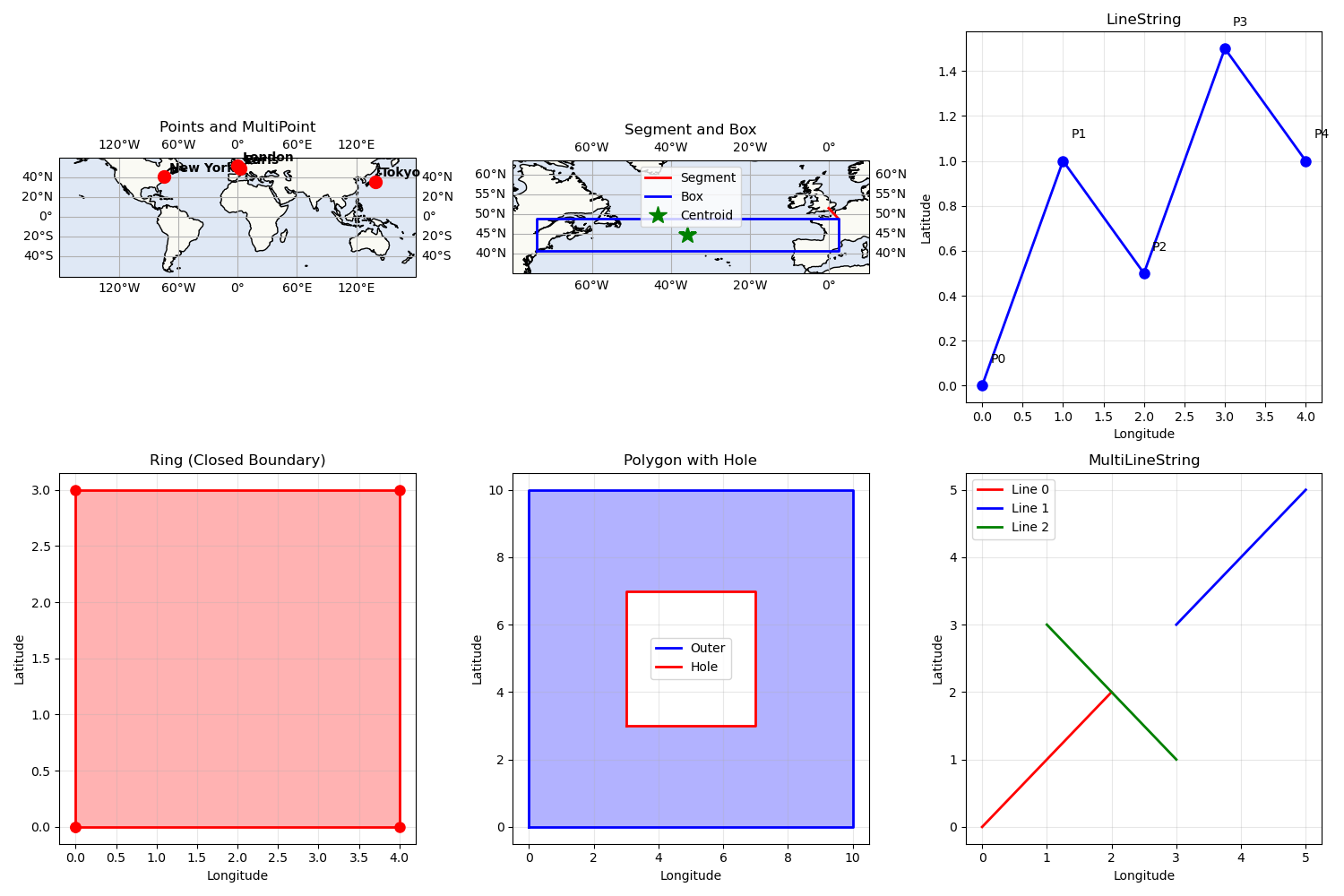
Visualizing Geometric Primitives

Let’s visualize some of the primitives we’ve created

fig = matplotlib.pyplot.figure(figsize=(15, 10))

# Plot 1: Points and MultiPoint
ax1 = fig.add_subplot(2, 3, 1, projection=cartopy.crs.PlateCarree())
ax1.add_feature(cartopy.feature.LAND, alpha=0.3)
ax1.add_feature(cartopy.feature.OCEAN, alpha=0.3)
ax1.add_feature(cartopy.feature.COASTLINE)
ax1.gridlines(draw_labels=True, dms=True, x_inline=False, y_inline=False)
ax1.set_extent([-180, 180, -60, 60])

# Plot cities
city_names = ["Paris", "New York", "London", "Tokyo"]
for city, name in zip(cities, city_names, strict=False):
    ax1.plot(
        city.lon,
        city.lat,
        "ro",
        markersize=10,
        transform=cartopy.crs.PlateCarree(),
        zorder=5,
    )
    ax1.text(
        city.lon + 5,
        city.lat + 5,
        name,
        transform=cartopy.crs.PlateCarree(),
        fontsize=10,
        fontweight="bold",
    )

ax1.set_title("Points and MultiPoint")

# Plot 2: Segment and Box
ax2 = fig.add_subplot(2, 3, 2, projection=cartopy.crs.PlateCarree())
ax2.add_feature(cartopy.feature.LAND, alpha=0.3)
ax2.add_feature(cartopy.feature.OCEAN, alpha=0.3)
ax2.add_feature(cartopy.feature.COASTLINE)
ax2.gridlines(draw_labels=True, dms=True, x_inline=False, y_inline=False)
ax2.set_extent([-80, 10, 35, 55])

# Plot segment
ax2.plot(
    *segment.to_arrays(),
    "r-",
    linewidth=2,
    label="Segment",
    transform=cartopy.crs.PlateCarree(),
)

# Plot box
box_lon, box_lat = geographic.algorithms.transform_to_polygon(
    box
).outer.to_arrays()
ax2.plot(
    box_lon,
    box_lat,
    "b-",
    linewidth=2,
    label="Box",
    transform=cartopy.crs.PlateCarree(),
)
ax2.plot(
    centroid.lon,
    centroid.lat,
    "g*",
    markersize=15,
    label="Centroid",
    transform=cartopy.crs.PlateCarree(),
)

ax2.legend()
ax2.set_title("Segment and Box")

# Plot 3: LineString
ax3 = fig.add_subplot(2, 3, 3)
ax3.plot(lon_array, lat_array, "bo-", linewidth=2, markersize=8)
for i, (lon, lat) in enumerate(zip(lon_array, lat_array, strict=False)):
    ax3.text(lon + 0.1, lat + 0.1, f"P{i}", fontsize=10)
ax3.grid(True, alpha=0.3)
ax3.set_xlabel("Longitude")
ax3.set_ylabel("Latitude")
ax3.set_title("LineString")

# Plot 4: Ring
ax4 = fig.add_subplot(2, 3, 4)
ax4.plot(ring_lon, ring_lat, "ro-", linewidth=2, markersize=8)
ax4.fill(ring_lon, ring_lat, alpha=0.3, color="red")
ax4.grid(True, alpha=0.3)
ax4.set_xlabel("Longitude")
ax4.set_ylabel("Latitude")
ax4.set_title("Ring (Closed Boundary)")

# Plot 5: Polygon with Hole
ax5 = fig.add_subplot(2, 3, 5)
ax5.plot(outer_lon, outer_lat, "b-", linewidth=2, label="Outer")
ax5.fill(outer_lon, outer_lat, alpha=0.3, color="blue")
ax5.plot(hole_lon, hole_lat, "r-", linewidth=2, label="Hole")
ax5.fill(hole_lon, hole_lat, alpha=1.0, color="white")
ax5.grid(True, alpha=0.3)
ax5.set_xlabel("Longitude")
ax5.set_ylabel("Latitude")
ax5.set_title("Polygon with Hole")
ax5.legend()

# Plot 6: MultiLineString
ax6 = fig.add_subplot(2, 3, 6)
colors = ["red", "blue", "green"]
for i, (line, color) in enumerate(zip(multiline, colors, strict=False)):
    lons = [pt.lon for pt in line]
    lats = [pt.lat for pt in line]
    ax6.plot(lons, lats, f"{color}", linewidth=2, label=f"Line {i}")
ax6.grid(True, alpha=0.3)
ax6.set_xlabel("Longitude")
ax6.set_ylabel("Latitude")
ax6.set_title("MultiLineString")
ax6.legend()

matplotlib.pyplot.tight_layout()