Drift paths from geostrophic velocity fields (path)

This example reproduces, in a compact and executable form, the workflow documented in the console script guide for path (see [docs/source/scripts/path.rst](https://cnes.github.io/aviso-lagrangian/scripts/path.html)). It shows how to:

• Build the configuration of a velocity time series from a list of NetCDF files (using the same template as in tests/map.ini)

• Run the console entry-point programmatically to compute the trajectories of a set of points listed in tests/buoys.txt

• Inspect the ASCII output and display the trajectories on a simple plot

Input and configuration

We propagate a small set of points from 2010-01-01 to 2010-01-02 using the built-in test dataset. The configuration uses the same template as in the documentation and the unit tests, relying on an environment variable ROOT to locate the test data folder.

from __future__ import annotations

import csv
import os
import pathlib
import sys
import tempfile
from collections import defaultdict
from datetime import datetime

import matplotlib.pyplot as plt

import lagrangian

# The console script we want to run programmatically
from lagrangian.console_scripts.path import main as path_main

Define the ROOT folder of this example (the examples directory)

EXAMPLES_DIRECTORY_PATH = pathlib.Path().absolute()

Define the base directory for tests data (used by SampleDataHandler)

TESTS_DIRECTORY_PATH = EXAMPLES_DIRECTORY_PATH.parent / 'tests'

Use the built-in test data provided by the lagrangian library, but store it in the tests folder so it can be reused by other gallery examples.

class SampleDataHandler(lagrangian.SampleDataHandler):
    ROOT = TESTS_DIRECTORY_PATH


# Download the built-in test data if not already present
SampleDataHandler()

<__main__.SampleDataHandler object at 0x7f6932817c50>

Prepare the configuration and input files (reusing tests/map.ini and tests/buoys.txt). The configuration relies on ${ROOT}, which we set to the built-in test data folder.

os.environ['ROOT'] = str(SampleDataHandler.folder())
map_ini_path = TESTS_DIRECTORY_PATH / 'map.ini'
buoys_txt_path = TESTS_DIRECTORY_PATH / 'buoys.txt'

Define the output ASCII file path for the trajectories

out_txt = pathlib.Path(tempfile.gettempdir()) / 'paths_gallery.txt'

Define the command line arguments to run the console script

sys.argv = [
    'path',
    str(map_ini_path),
    str(buoys_txt_path),
    '2010-01-01',
    '2010-01-02',
    '--output',
    str(out_txt),
]

Run the console script programmatically

path_main()

Load the generated ASCII output. The format is tab-separated with 4 columns: index, longitude, latitude, ISO8601 timestamp. We’ll parse it and show the first few entries for inspection.

rows: list[tuple[int, float, float, datetime]] = []
with open(out_txt) as f:
    reader = csv.reader(f, delimiter='\t')
    for idx_str, lon_str, lat_str, ts_str in reader:
        rows.append((
            int(idx_str),
            float(lon_str),
            float(lat_str),
            datetime.fromisoformat(ts_str),
        ))

print('Preview of path output (first 10 lines):')
for r in rows[:10]:
    print(f"{r[0]}\t{r[1]:.6f}\t{r[2]:.6f}\t{r[3].isoformat()}")

Preview of path output (first 10 lines):
0       0.000000        0.000000        2010-01-01T00:00:00
1       1.433333        43.600000       2010-01-01T00:00:00
2       2.000000        2.000000        2010-01-01T00:00:00
3       4.000000        4.000000        2010-01-01T00:00:00
4       8.000000        8.000000        2010-01-01T00:00:00
5       16.000000       16.000000       2010-01-01T00:00:00
6       32.000000       32.000000       2010-01-01T00:00:00
7       64.000000       64.000000       2010-01-01T00:00:00
8       70.000000       12.000000       2010-01-01T00:00:00
0       -0.038031       -0.013479       2010-01-01T06:00:00

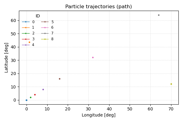
Plot trajectories by connecting positions for each particle index. This is a simple geographic plot in lon/lat without map projection for brevity.

tracks: dict[int, list[tuple[float, float]]] = defaultdict(list)
for pid, lon, lat, _ in rows:
    tracks[pid].append((lon, lat))

fig, ax = plt.subplots(figsize=(6, 4))
for pid, pts in sorted(tracks.items()):
    if not pts:
        continue
    xs, ys = zip(*pts)
    ax.plot(xs, ys, marker='o', markersize=2, linewidth=1, label=str(pid))

ax.set_title('Particle trajectories (path)')
ax.set_xlabel('Longitude [deg]')
ax.set_ylabel('Latitude [deg]')
ax.legend(title='ID',
          loc='upper left',
          ncol=2,
          fontsize='small',
          frameon=False)
ax.grid(True, linestyle=':', linewidth=0.5)
plt.tight_layout()