Quickstart#
Now that you installation went ok, let’s start with a small example. Let’s create our first Geodes object.
[1]:
from pygeodes import Geodes

geodes = Geodes()
Searching for collections#
Then we can start by searching for existing collections, for example with search term sentinel :
[2]:
collections, dataframe = geodes.search_collections("sentinel")
/work/scratch/data/robertm/dev/env_tmp/pygeodes_cible/lib/python3.11/site-packages/urllib3/connectionpool.py:1097: InsecureRequestWarning: Unverified HTTPS request is being made to host 'geodes-portal.cnes.fr'. Adding certificate verification is strongly advised. See: https://urllib3.readthedocs.io/en/latest/advanced-usage.html#tls-warnings
  warnings.warn(
Indexing: 100%|██████████| 66/66 [00:00<00:00, 2867.81it/s]
Let’s see what we found. As a result, we get a collections object, which is a list of Collection objects.
[3]:
collections
[3]:
[<Collection id=THEIA_S1TILING_SENTINEL1_L1>,
 <Collection id=THEIA_BIOPHY_SENTINEL2_L2B>,
 <Collection id=THEIA_WATERQUAL_SENTINEL2_L2B>,
 <Collection id=THEIA_REFLECTANCE_SENTINEL2_L3A>,
 <Collection id=THEIA_REFLECTANCE_SENTINEL2_L2A>,
 <Collection id=PEPS_S2_L1C>,
 <Collection id=PEPS_S1_L2>,
 <Collection id=PEPS_S1_L1>,
 <Collection id=THEIA_SPOT4_TAKE5_L1C>,
 <Collection id=THEIA_REFLECTANCE_LANDSAT8_L2A>,
 <Collection id=THEIA_OSO_RASTER_L3B>,
 <Collection id=THEIA_REFLECTANCE_SPOT4_TAKE5_L2A>,
 <Collection id=PEPS_S3_L1>,
 <Collection id=THEIA_SPOT5_TAKE5_L1C>,
 <Collection id=THEIA_REFLECTANCE_SPOT5_TAKE5_L2A>,
 <Collection id=THEIA_OSO_VECTOR_L3B>]
and a dataframe object, which is a geopandas.GeoDataFrame.
[4]:
dataframe
[4]:
| title | description | collection | |
|---|---|---|---|
| 0 | THEIA S1TILING SENTINEL L1 | S1TILING L1 products are based on Sentinel-1 L... | <Collection id=THEIA_S1TILING_SENTINEL1_L1> |
| 1 | THEIA SENTINEL2 BIOPHY L2B | Biophysical variables characteristic of vegeta... | <Collection id=THEIA_BIOPHY_SENTINEL2_L2B> |
| 2 | THEIA WaterQual SENTINEL2 L2B | The processing chain outputs rasters of the co... | <Collection id=THEIA_WATERQUAL_SENTINEL2_L2B> |
| 3 | THEIA SENTINEL2 L3A | The products of level 3A provide a monthly syn... | <Collection id=THEIA_REFLECTANCE_SENTINEL2_L3A> |
| 4 | THEIA SENTINEL2 L2A | The level 2A products correct the data for atm... | <Collection id=THEIA_REFLECTANCE_SENTINEL2_L2A> |
| 5 | PEPS Sentinel-2 L1C tiles | Sentinel-2 L1C tiles acquisition and storage f... | <Collection id=PEPS_S2_L1C> |
| 6 | PEPS Sentinel-1 Level2 | Sentinel-1 Level-2 consists of geolocated geop... | <Collection id=PEPS_S1_L2> |
| 7 | PEPS Sentinel-1 Level1 | Sentinel-1 Level-1 products are the baseline p... | <Collection id=PEPS_S1_L1> |
| 8 | TAKE5 SPOT4 LEVEL1C | At the end of life of each satellite, CNES iss... | <Collection id=THEIA_SPOT4_TAKE5_L1C> |
| 9 | THEIA LANDSAT8 L2A | The level 2A products correct the data for atm... | <Collection id=THEIA_REFLECTANCE_LANDSAT8_L2A> |
| 10 | THEIA OSO RASTER | Main characteristics of the OSO Land Cover pro... | <Collection id=THEIA_OSO_RASTER_L3B> |
| 11 | TAKE5 SPOT4 LEVEL2A | At the end of life of each satellite, CNES iss... | <Collection id=THEIA_REFLECTANCE_SPOT4_TAKE5_L2A> |
| 12 | GDH Sentinel-3 L1 STM Level-1 products | Sea surface topography measurements to at leas... | <Collection id=PEPS_S3_L1> |
| 13 | TAKE5 SPOT5 LEVEL1C | At the end of life of each satellite, CNES iss... | <Collection id=THEIA_SPOT5_TAKE5_L1C> |
| 14 | TAKE5 SPOT5 LEVEL2A | At the end of life of each satellite, CNES iss... | <Collection id=THEIA_REFLECTANCE_SPOT5_TAKE5_L2A> |
| 15 | THEIA OSO VECTOR | Main characteristics of the OSO Land Cover pro... | <Collection id=THEIA_OSO_VECTOR_L3B> |
The dataframe let’s see you quickly see what you found, with only a few columns (here description and title), but if you are more comfortable working with raw objects, it’s also possible.
Let’s see how many elements are in these collections.
[5]:
for collection in collections:
    print(
        f"collection {collection.title} has {collection.summaries.other.get('total_items')} elements"
    )
collection THEIA S1TILING SENTINEL L1 has 0 elements
collection THEIA SENTINEL2 BIOPHY L2B has 0 elements
collection THEIA WaterQual SENTINEL2 L2B has 138 elements
collection THEIA SENTINEL2 L3A has 63568 elements
collection THEIA SENTINEL2 L2A has 2177670 elements
collection PEPS Sentinel-2 L1C tiles has 37010592 elements
collection PEPS Sentinel-1 Level2 has 1534336 elements
collection PEPS Sentinel-1 Level1 has 6441578 elements
collection TAKE5 SPOT4 LEVEL1C has 902 elements
collection THEIA LANDSAT8 L2A has 27896 elements
collection THEIA OSO RASTER has 9 elements
collection TAKE5 SPOT4 LEVEL2A has 814 elements
collection GDH Sentinel-3 L1 STM Level-1 products has 64805 elements
collection TAKE5 SPOT5 LEVEL1C has 3740 elements
collection TAKE5 SPOT5 LEVEL2A has 2953 elements
collection THEIA OSO VECTOR has 864 elements
We could want to add columns to our dataframe. To know which columns are available, use collection.list_available_keys() on a Collection object :
[6]:
collections[0].list_available_keys()
[6]:
{'assets.bs.description',
 'assets.bs.href',
 'assets.bs.roles',
 'assets.bs.title',
 'assets.bs.type',
 'assets.wms_capabilities.description',
 'assets.wms_capabilities.href',
 'assets.wms_capabilities.roles',
 'assets.wms_capabilities.title',
 'assets.wms_capabilities.type',
 'description',
 'extent.spatial.bbox',
 'extent.temporal.interval',
 'id',
 'keywords',
 'license',
 'links',
 'providers',
 'stac_extensions',
 'stac_version',
 'summaries.access_url',
 'summaries.constellation',
 'summaries.contact_email',
 'summaries.contact_name',
 'summaries.dataset',
 'summaries.format',
 'summaries.geometry_type',
 'summaries.gsd',
 'summaries.instruments',
 'summaries.item_type',
 'summaries.latest',
 'summaries.missions',
 'summaries.platform',
 'summaries.processing:level',
 'summaries.production_frequency',
 'summaries.temporal_resolution',
 'summaries.theme',
 'summaries.total_items',
 'summaries.variables',
 'summaries.version',
 'title',
 'type'}
Let’s add summaries.total_items to the dataframe :
[7]:
from pygeodes.utils.formatting import format_collections

new_dataframe = format_collections(
    dataframe, columns_to_add={"summaries.total_items"}
)
[8]:
new_dataframe
[8]:
| title | description | collection | summaries.total_items | |
|---|---|---|---|---|
| 0 | THEIA S1TILING SENTINEL L1 | S1TILING L1 products are based on Sentinel-1 L... | <Collection id=THEIA_S1TILING_SENTINEL1_L1> | 0 |
| 1 | THEIA SENTINEL2 BIOPHY L2B | Biophysical variables characteristic of vegeta... | <Collection id=THEIA_BIOPHY_SENTINEL2_L2B> | 0 |
| 2 | THEIA WaterQual SENTINEL2 L2B | The processing chain outputs rasters of the co... | <Collection id=THEIA_WATERQUAL_SENTINEL2_L2B> | 138 |
| 3 | THEIA SENTINEL2 L3A | The products of level 3A provide a monthly syn... | <Collection id=THEIA_REFLECTANCE_SENTINEL2_L3A> | 63568 |
| 4 | THEIA SENTINEL2 L2A | The level 2A products correct the data for atm... | <Collection id=THEIA_REFLECTANCE_SENTINEL2_L2A> | 2177670 |
| 5 | PEPS Sentinel-2 L1C tiles | Sentinel-2 L1C tiles acquisition and storage f... | <Collection id=PEPS_S2_L1C> | 37010592 |
| 6 | PEPS Sentinel-1 Level2 | Sentinel-1 Level-2 consists of geolocated geop... | <Collection id=PEPS_S1_L2> | 1534336 |
| 7 | PEPS Sentinel-1 Level1 | Sentinel-1 Level-1 products are the baseline p... | <Collection id=PEPS_S1_L1> | 6441578 |
| 8 | TAKE5 SPOT4 LEVEL1C | At the end of life of each satellite, CNES iss... | <Collection id=THEIA_SPOT4_TAKE5_L1C> | 902 |
| 9 | THEIA LANDSAT8 L2A | The level 2A products correct the data for atm... | <Collection id=THEIA_REFLECTANCE_LANDSAT8_L2A> | 27896 |
| 10 | THEIA OSO RASTER | Main characteristics of the OSO Land Cover pro... | <Collection id=THEIA_OSO_RASTER_L3B> | 9 |
| 11 | TAKE5 SPOT4 LEVEL2A | At the end of life of each satellite, CNES iss... | <Collection id=THEIA_REFLECTANCE_SPOT4_TAKE5_L2A> | 814 |
| 12 | GDH Sentinel-3 L1 STM Level-1 products | Sea surface topography measurements to at leas... | <Collection id=PEPS_S3_L1> | 64805 |
| 13 | TAKE5 SPOT5 LEVEL1C | At the end of life of each satellite, CNES iss... | <Collection id=THEIA_SPOT5_TAKE5_L1C> | 3740 |
| 14 | TAKE5 SPOT5 LEVEL2A | At the end of life of each satellite, CNES iss... | <Collection id=THEIA_REFLECTANCE_SPOT5_TAKE5_L2A> | 2953 |
| 15 | THEIA OSO VECTOR | Main characteristics of the OSO Land Cover pro... | <Collection id=THEIA_OSO_VECTOR_L3B> | 864 |
If you wish to produce a fresh new dataframe with your custom columns, use format_collections on a list of collections :
[9]:
new_dataframe = format_collections(
    collections,
    columns_to_add={"summaries.constellation", "summaries.instruments"},
)
[10]:
new_dataframe
[10]:
| summaries.constellation | summaries.instruments | title | description | collection | |
|---|---|---|---|---|---|
| 0 | [sentinel-1] | [SAR] | THEIA S1TILING SENTINEL L1 | S1TILING L1 products are based on Sentinel-1 L... | <Collection id=THEIA_S1TILING_SENTINEL1_L1> |
| 1 | [sentinel-2] | [MSI] | THEIA SENTINEL2 BIOPHY L2B | Biophysical variables characteristic of vegeta... | <Collection id=THEIA_BIOPHY_SENTINEL2_L2B> |
| 2 | [sentinel-2] | [] | THEIA WaterQual SENTINEL2 L2B | The processing chain outputs rasters of the co... | <Collection id=THEIA_WATERQUAL_SENTINEL2_L2B> |
| 3 | [sentinel-2] | [MSI] | THEIA SENTINEL2 L3A | The products of level 3A provide a monthly syn... | <Collection id=THEIA_REFLECTANCE_SENTINEL2_L3A> |
| 4 | [sentinel-2] | [MSI] | THEIA SENTINEL2 L2A | The level 2A products correct the data for atm... | <Collection id=THEIA_REFLECTANCE_SENTINEL2_L2A> |
| 5 | [sentinel-2] | [MSI] | PEPS Sentinel-2 L1C tiles | Sentinel-2 L1C tiles acquisition and storage f... | <Collection id=PEPS_S2_L1C> |
| 6 | [sentinel-1] | [SAR-C] | PEPS Sentinel-1 Level2 | Sentinel-1 Level-2 consists of geolocated geop... | <Collection id=PEPS_S1_L2> |
| 7 | [sentinel-1] | [SAR-C] | PEPS Sentinel-1 Level1 | Sentinel-1 Level-1 products are the baseline p... | <Collection id=PEPS_S1_L1> |
| 8 | [spot-4] | [HRV, HRVIR] | TAKE5 SPOT4 LEVEL1C | At the end of life of each satellite, CNES iss... | <Collection id=THEIA_SPOT4_TAKE5_L1C> |
| 9 | [landsat-8] | [OLI] | THEIA LANDSAT8 L2A | The level 2A products correct the data for atm... | <Collection id=THEIA_REFLECTANCE_LANDSAT8_L2A> |
| 10 | [sentinel-2] | None | THEIA OSO RASTER | Main characteristics of the OSO Land Cover pro... | <Collection id=THEIA_OSO_RASTER_L3B> |
| 11 | [spot-4] | [HRV, HRVIR] | TAKE5 SPOT4 LEVEL2A | At the end of life of each satellite, CNES iss... | <Collection id=THEIA_REFLECTANCE_SPOT4_TAKE5_L2A> |
| 12 | [sentinel-3] | [SRAL] | GDH Sentinel-3 L1 STM Level-1 products | Sea surface topography measurements to at leas... | <Collection id=PEPS_S3_L1> |
| 13 | [spot-5] | [HRG1, HRG2] | TAKE5 SPOT5 LEVEL1C | At the end of life of each satellite, CNES iss... | <Collection id=THEIA_SPOT5_TAKE5_L1C> |
| 14 | [spot-5] | [HRG1, HRG2] | TAKE5 SPOT5 LEVEL2A | At the end of life of each satellite, CNES iss... | <Collection id=THEIA_REFLECTANCE_SPOT5_TAKE5_L2A> |
| 15 | [sentinel-2] | None | THEIA OSO VECTOR | Main characteristics of the OSO Land Cover pro... | <Collection id=THEIA_OSO_VECTOR_L3B> |
Note : title and description columns are always here by default.
Searching for items#
As for collections, we can search for items. To know which arguments to put in your query, please use :
[11]:
from pygeodes.utils.query import get_requestable_args

print(get_requestable_args())
{'version': 'v8.0', 'attributes': ['dataset (STRING)', 'datetime (DATE_ISO8601)', 'links (STRING)', 'product_validity (BOOLEAN)', 'sci:doi (STRING_ARRAY)', 'no_geometry (BOOLEAN)', 'start_datetime (DATE_ISO8601)', 'end_datetime (DATE_ISO8601)', 'processing:datetime (DATE_ISO8601)', 'processing:lineage (STRING)', 'processing_context (STRING)', 'processing_correction (STRING)', 'processing:version (STRING)', 'bbox (STRING)', 'nb_cols (STRING)', 'nb_rows (STRING)', 'instrument (STRING)', 'platform (STRING)', 'sar:instrument_mode (STRING)', 'processing:level (STRING)', 'sar:polarizations (STRING)', 'sat:orbit_cycle (INTEGER)', 'mission_take_id (INTEGER)', 's2:datatake_id (STRING)', 'sat:relative_orbit (INTEGER)', 'sat:absolute_orbit (LONG)', 'sat:orbit_state (STRING)', 'product:type (STRING)', 'parameter (STRING)', 'pparameter (STRING)', 'product (STRING)', 'temporal_resolution (STRING)', 'classification (STRING)', 'swath (STRING)', 'bands (STRING)', 'grid:code (STRING)', 'eo:cloud_cover (DOUBLE)', 'water_cover (DOUBLE)', 'saturated_defective_pixel (DOUBLE)', 'nodata_pixel (DOUBLE)', 'nb_col_interpolation_error (DOUBLE)', 'ground_useful_pixel (DOUBLE)', 'min_useful_pixel (DOUBLE)', 'sensor_angle (DOUBLE)', 'sensor_pitch (DOUBLE)', 'sensor_roll (DOUBLE)', 'continent_code (STRING_ARRAY)', 'area (DOUBLE)', 'sar:beam_ids (STRING)', 'subTile (STRING)', 'keywords (STRING_ARRAY)', 'political (JSON)']}
[12]:
query = {"sat:relative_orbit": {"eq": 4}}
sortBy = [{"direction":"desc","field":"start_datetime"}]
items, dataframe = geodes.search_items(query=query, sortBy=sortBy, collections=['PEPS_S2_L1C'])
/work/scratch/data/robertm/dev/env_tmp/pygeodes_cible/lib/python3.11/site-packages/urllib3/connectionpool.py:1097: InsecureRequestWarning: Unverified HTTPS request is being made to host 'geodes-portal.cnes.fr'. Adding certificate verification is strongly advised. See: https://urllib3.readthedocs.io/en/latest/advanced-usage.html#tls-warnings
  warnings.warn(
Found 258470 items matching your query, returning 80 as get_all parameter is set to False
80 item(s) found for query : {'sat:relative_orbit': {'eq': 4}}
Again, we come out with an items object, and a dataframe object.
[13]:
items[:10] # printing everything is useless
[13]:
[Item (URN:FEATURE:DATA:gdh:8f917459-f72f-341c-a713-ca7f0ff0f01e:V1),
 Item (URN:FEATURE:DATA:gdh:c052606a-1e73-37c8-8de6-506412807a08:V1),
 Item (URN:FEATURE:DATA:gdh:cbdbb19f-5cc3-3af2-8d83-7f7248720e16:V1),
 Item (URN:FEATURE:DATA:gdh:0811550e-7f8a-3582-a8e6-202b9a73afdd:V1),
 Item (URN:FEATURE:DATA:gdh:219ec988-7c8f-3fac-8f9e-661d919563f0:V1),
 Item (URN:FEATURE:DATA:gdh:11eebd44-01fd-3089-8d1c-2ce0a4d0b6fe:V1),
 Item (URN:FEATURE:DATA:gdh:ec36c006-0b3a-36c3-9f46-69f2f3be8ab8:V1),
 Item (URN:FEATURE:DATA:gdh:0d56d04e-1f05-3bae-9ada-1deef90a9ba0:V1),
 Item (URN:FEATURE:DATA:gdh:3b46df15-8955-35b4-a3e4-a6ba178c1d4c:V1),
 Item (URN:FEATURE:DATA:gdh:71c19643-9924-3684-810f-58c5432cdcf8:V1)]
[14]:
dataframe
[14]:
| id | sat:relative_orbit | collection | item | geometry | |
|---|---|---|---|---|---|
| 0 | URN:FEATURE:DATA:gdh:8f917459-f72f-341c-a713-c... | 4 | PEPS_S2_L1C | Item (URN:FEATURE:DATA:gdh:8f917459-f72f-341c-... | POLYGON ((96.19312 16.26222, 96.20672 15.27075... |
| 1 | URN:FEATURE:DATA:gdh:c052606a-1e73-37c8-8de6-5... | 4 | PEPS_S2_L1C | Item (URN:FEATURE:DATA:gdh:c052606a-1e73-37c8-... | POLYGON ((103.08352 45.94729, 103.83596 45.959... |
| 2 | URN:FEATURE:DATA:gdh:cbdbb19f-5cc3-3af2-8d83-7... | 4 | PEPS_S2_L1C | Item (URN:FEATURE:DATA:gdh:cbdbb19f-5cc3-3af2-... | POLYGON ((101.5455 38.79789, 101.59209 37.8101... |
| 3 | URN:FEATURE:DATA:gdh:0811550e-7f8a-3582-a8e6-2... | 4 | PEPS_S2_L1C | Item (URN:FEATURE:DATA:gdh:0811550e-7f8a-3582-... | POLYGON ((101.24793 37.02528, 101.21947 36.036... |
| 4 | URN:FEATURE:DATA:gdh:219ec988-7c8f-3fac-8f9e-6... | 4 | PEPS_S2_L1C | Item (URN:FEATURE:DATA:gdh:219ec988-7c8f-3fac-... | POLYGON ((107.79861 47.73874, 107.80285 47.819... |
| ... | ... | ... | ... | ... | ... |
| 75 | URN:FEATURE:DATA:gdh:4c758d19-7362-3e27-812b-5... | 4 | PEPS_S2_L1C | Item (URN:FEATURE:DATA:gdh:4c758d19-7362-3e27-... | POLYGON ((104.99971 51.04807, 104.99972 50.463... |
| 76 | URN:FEATURE:DATA:gdh:59d3bc97-c0e2-308d-94ab-2... | 4 | PEPS_S2_L1C | Item (URN:FEATURE:DATA:gdh:59d3bc97-c0e2-308d-... | POLYGON ((101.45454 40.5964, 101.50549 39.6090... |
| 77 | URN:FEATURE:DATA:gdh:8c9455d5-9faf-31bc-bafd-8... | 4 | PEPS_S2_L1C | Item (URN:FEATURE:DATA:gdh:8c9455d5-9faf-31bc-... | POLYGON ((114.81208 65.80592, 114.89231 64.821... |
| 78 | URN:FEATURE:DATA:gdh:ccd73d19-4604-3d80-8bd6-8... | 4 | PEPS_S2_L1C | Item (URN:FEATURE:DATA:gdh:ccd73d19-4604-3d80-... | POLYGON ((101.43771 40.90608, 101.45918 40.508... |
| 79 | URN:FEATURE:DATA:gdh:0939f7e3-f40e-31c9-b6c3-8... | 4 | PEPS_S2_L1C | Item (URN:FEATURE:DATA:gdh:0939f7e3-f40e-31c9-... | POLYGON ((111.06215 54.14751, 109.46869 54.138... |
80 rows × 5 columns
Let’s have a look around our items.
A thing we could want to do is filter them by cloud cover, let’s say between 39 and 40. But this column doesn’t appear in the dataframe. To know which columns are available, use item.list_available_keys() on an Item object.
[15]:
items[0].list_available_keys()
[15]:
{'area',
 'continent_code',
 'dataset',
 'datetime',
 'end_datetime',
 'endpoint_description',
 'endpoint_url',
 'eo:cloud_cover',
 'grid:code',
 'id',
 'identifier',
 'instrument',
 'keywords',
 'latest',
 'physical',
 'platform',
 'political.continents',
 'processing:level',
 'product:timeliness',
 'product:type',
 'proj:bbox',
 'references',
 's2:datatake_id',
 'sar:instrument_mode',
 'sat:absolute_orbit',
 'sat:orbit_state',
 'sat:relative_orbit',
 'sci:doi',
 'start_datetime'}
We see we can use eo:cloud_cover. We can add it using format_items.
[16]:
from pygeodes.utils.formatting import format_items

new_dataframe = format_items(
    dataframe, columns_to_add={"eo:cloud_cover"}
)
[17]:
new_dataframe
[17]:
| id | sat:relative_orbit | collection | item | geometry | eo:cloud_cover | |
|---|---|---|---|---|---|---|
| 0 | URN:FEATURE:DATA:gdh:8f917459-f72f-341c-a713-c... | 4 | PEPS_S2_L1C | Item (URN:FEATURE:DATA:gdh:8f917459-f72f-341c-... | POLYGON ((96.19312 16.26222, 96.20672 15.27075... | 76.241363 |
| 1 | URN:FEATURE:DATA:gdh:c052606a-1e73-37c8-8de6-5... | 4 | PEPS_S2_L1C | Item (URN:FEATURE:DATA:gdh:c052606a-1e73-37c8-... | POLYGON ((103.08352 45.94729, 103.83596 45.959... | 0.256226 |
| 2 | URN:FEATURE:DATA:gdh:cbdbb19f-5cc3-3af2-8d83-7... | 4 | PEPS_S2_L1C | Item (URN:FEATURE:DATA:gdh:cbdbb19f-5cc3-3af2-... | POLYGON ((101.5455 38.79789, 101.59209 37.8101... | 0.000000 |
| 3 | URN:FEATURE:DATA:gdh:0811550e-7f8a-3582-a8e6-2... | 4 | PEPS_S2_L1C | Item (URN:FEATURE:DATA:gdh:0811550e-7f8a-3582-... | POLYGON ((101.24793 37.02528, 101.21947 36.036... | 0.019051 |
| 4 | URN:FEATURE:DATA:gdh:219ec988-7c8f-3fac-8f9e-6... | 4 | PEPS_S2_L1C | Item (URN:FEATURE:DATA:gdh:219ec988-7c8f-3fac-... | POLYGON ((107.79861 47.73874, 107.80285 47.819... | 0.009339 |
| ... | ... | ... | ... | ... | ... | ... |
| 75 | URN:FEATURE:DATA:gdh:4c758d19-7362-3e27-812b-5... | 4 | PEPS_S2_L1C | Item (URN:FEATURE:DATA:gdh:4c758d19-7362-3e27-... | POLYGON ((104.99971 51.04807, 104.99972 50.463... | 14.084793 |
| 76 | URN:FEATURE:DATA:gdh:59d3bc97-c0e2-308d-94ab-2... | 4 | PEPS_S2_L1C | Item (URN:FEATURE:DATA:gdh:59d3bc97-c0e2-308d-... | POLYGON ((101.45454 40.5964, 101.50549 39.6090... | 0.431813 |
| 77 | URN:FEATURE:DATA:gdh:8c9455d5-9faf-31bc-bafd-8... | 4 | PEPS_S2_L1C | Item (URN:FEATURE:DATA:gdh:8c9455d5-9faf-31bc-... | POLYGON ((114.81208 65.80592, 114.89231 64.821... | 99.982412 |
| 78 | URN:FEATURE:DATA:gdh:ccd73d19-4604-3d80-8bd6-8... | 4 | PEPS_S2_L1C | Item (URN:FEATURE:DATA:gdh:ccd73d19-4604-3d80-... | POLYGON ((101.43771 40.90608, 101.45918 40.508... | 29.061980 |
| 79 | URN:FEATURE:DATA:gdh:0939f7e3-f40e-31c9-b6c3-8... | 4 | PEPS_S2_L1C | Item (URN:FEATURE:DATA:gdh:0939f7e3-f40e-31c9-... | POLYGON ((111.06215 54.14751, 109.46869 54.138... | 76.702719 |
80 rows × 6 columns
We’ve got our new dataframe. Let’s filter :
[18]:
filtered = new_dataframe[
    (new_dataframe["eo:cloud_cover"] <= 30)
    & (new_dataframe["eo:cloud_cover"] >= 29)
]
[19]:
filtered
[19]:
| id | sat:relative_orbit | collection | item | geometry | eo:cloud_cover | |
|---|---|---|---|---|---|---|
| 78 | URN:FEATURE:DATA:gdh:ccd73d19-4604-3d80-8bd6-8... | 4 | PEPS_S2_L1C | Item (URN:FEATURE:DATA:gdh:ccd73d19-4604-3d80-... | POLYGON ((101.43771 40.90608, 101.45918 40.508... | 29.06198 |
Let’s plot these items :
[20]:
##Folim is required for the command below. You can install in your Python environment by executing pip install "folium>=0.12" matplotlib mapclassify
m = filtered.explore()
[21]:
m
[21]:
If you want to have all available columns in your dataframe, just do :
[22]:
full_dataframe = format_items(
    items, columns_to_add=items[0].list_available_keys()
)
[23]:
full_dataframe
[23]:
| id | proj:bbox | endpoint_description | collection | sat:orbit_state | product:timeliness | political.continents | product:type | processing:level | endpoint_url | ... | references | grid:code | identifier | eo:cloud_cover | sar:instrument_mode | keywords | end_datetime | start_datetime | item | geometry | |
|---|---|---|---|---|---|---|---|---|---|---|---|---|---|---|---|---|---|---|---|---|---|
| 0 | URN:FEATURE:DATA:gdh:8f917459-f72f-341c-a713-c... | Link to product in datalake | PEPS_S2_L1C | Descending | Nominal | [] | S2MSI1C | L1C | https://s3.datalake.cnes.fr/sentinel2-l1c/47/P... | ... | [{'url': 'http://www.naturalearthdata.com/down... | T47PKT | S2C_MSIL1C_20260215T035841_N0512_R004_T47PKT_2... | 76.241363 | INS-NOBS | [location:tropical, location:northern, season:... | 2026-02-15T03:58:41.025Z | 2026-02-15T03:58:41.025Z | Item (URN:FEATURE:DATA:gdh:8f917459-f72f-341c-... | POLYGON ((96.19312 16.26222, 96.20672 15.27075... | |
| 1 | URN:FEATURE:DATA:gdh:c052606a-1e73-37c8-8de6-5... | Link to product in datalake | PEPS_S2_L1C | Descending | Nominal | [{'id': 'continent:Asia:6255147', 'name': 'Asi... | S2MSI1C | L1C | https://s3.datalake.cnes.fr/sentinel2-l1c/48/T... | ... | [{'url': 'http://www.naturalearthdata.com/down... | T48TUS | S2C_MSIL1C_20260215T035841_N0512_R004_T48TUS_2... | 0.256226 | INS-NOBS | [location:northern, season:winter] | 2026-02-15T03:58:41.025Z | 2026-02-15T03:58:41.025Z | Item (URN:FEATURE:DATA:gdh:c052606a-1e73-37c8-... | POLYGON ((103.08352 45.94729, 103.83596 45.959... | |
| 2 | URN:FEATURE:DATA:gdh:cbdbb19f-5cc3-3af2-8d83-7... | Link to product in datalake | PEPS_S2_L1C | Descending | Nominal | [{'id': 'continent:Asia:6255147', 'name': 'Asi... | S2MSI1C | L1C | https://s3.datalake.cnes.fr/sentinel2-l1c/48/S... | ... | [{'url': 'http://www.naturalearthdata.com/down... | T48STH | S2C_MSIL1C_20260215T035841_N0512_R004_T48STH_2... | 0.000000 | INS-NOBS | [location:northern, season:winter] | 2026-02-15T03:58:41.025Z | 2026-02-15T03:58:41.025Z | Item (URN:FEATURE:DATA:gdh:cbdbb19f-5cc3-3af2-... | POLYGON ((101.5455 38.79789, 101.59209 37.8101... | |
| 3 | URN:FEATURE:DATA:gdh:0811550e-7f8a-3582-a8e6-2... | Link to product in datalake | PEPS_S2_L1C | Descending | Nominal | [{'id': 'continent:Asia:6255147', 'name': 'Asi... | S2MSI1C | L1C | https://s3.datalake.cnes.fr/sentinel2-l1c/47/S... | ... | [{'url': 'http://www.naturalearthdata.com/down... | T47SQA | S2C_MSIL1C_20260215T035841_N0512_R004_T47SQA_2... | 0.019051 | INS-NOBS | [location:northern, season:winter] | 2026-02-15T03:58:41.025Z | 2026-02-15T03:58:41.025Z | Item (URN:FEATURE:DATA:gdh:0811550e-7f8a-3582-... | POLYGON ((101.24793 37.02528, 101.21947 36.036... | |
| 4 | URN:FEATURE:DATA:gdh:219ec988-7c8f-3fac-8f9e-6... | Link to product in datalake | PEPS_S2_L1C | Descending | Nominal | [{'id': 'continent:Asia:6255147', 'name': 'Asi... | S2MSI1C | L1C | https://s3.datalake.cnes.fr/sentinel2-l1c/48/T... | ... | [{'url': 'http://www.naturalearthdata.com/down... | T48TXT | S2C_MSIL1C_20260215T035841_N0512_R004_T48TXT_2... | 0.009339 | INS-NOBS | [location:northern, season:winter] | 2026-02-15T03:58:41.025Z | 2026-02-15T03:58:41.025Z | Item (URN:FEATURE:DATA:gdh:219ec988-7c8f-3fac-... | POLYGON ((107.79861 47.73874, 107.80285 47.819... | |
| ... | ... | ... | ... | ... | ... | ... | ... | ... | ... | ... | ... | ... | ... | ... | ... | ... | ... | ... | ... | ... | ... |
| 75 | URN:FEATURE:DATA:gdh:4c758d19-7362-3e27-812b-5... | Link to product in datalake | PEPS_S2_L1C | Descending | Nominal | [{'id': 'continent:Europe:6255148', 'name': 'E... | S2MSI1C | L1C | https://s3.datalake.cnes.fr/sentinel2-l1c/48/U... | ... | [{'url': 'http://www.naturalearthdata.com/down... | T48UWB | S2C_MSIL1C_20260215T035841_N0512_R004_T48UWB_2... | 14.084793 | INS-NOBS | [location:northern, season:winter] | 2026-02-15T03:58:41.025Z | 2026-02-15T03:58:41.025Z | Item (URN:FEATURE:DATA:gdh:4c758d19-7362-3e27-... | POLYGON ((104.99971 51.04807, 104.99972 50.463... | |
| 76 | URN:FEATURE:DATA:gdh:59d3bc97-c0e2-308d-94ab-2... | Link to product in datalake | PEPS_S2_L1C | Descending | Nominal | [{'id': 'continent:Asia:6255147', 'name': 'Asi... | S2MSI1C | L1C | https://s3.datalake.cnes.fr/sentinel2-l1c/48/T... | ... | [{'url': 'http://www.naturalearthdata.com/down... | T48TTK | S2C_MSIL1C_20260215T035841_N0512_R004_T48TTK_2... | 0.431813 | INS-NOBS | [location:northern, season:winter] | 2026-02-15T03:58:41.025Z | 2026-02-15T03:58:41.025Z | Item (URN:FEATURE:DATA:gdh:59d3bc97-c0e2-308d-... | POLYGON ((101.45454 40.5964, 101.50549 39.6090... | |
| 77 | URN:FEATURE:DATA:gdh:8c9455d5-9faf-31bc-bafd-8... | Link to product in datalake | PEPS_S2_L1C | Descending | Nominal | [{'id': 'continent:Europe:6255148', 'name': 'E... | S2MSI1C | L1C | https://s3.datalake.cnes.fr/sentinel2-l1c/50/W... | ... | [{'url': 'http://www.naturalearthdata.com/down... | T50WMT | S2C_MSIL1C_20260215T035841_N0512_R004_T50WMT_2... | 99.982412 | INS-NOBS | [location:northern, season:winter] | 2026-02-15T03:58:41.025Z | 2026-02-15T03:58:41.025Z | Item (URN:FEATURE:DATA:gdh:8c9455d5-9faf-31bc-... | POLYGON ((114.81208 65.80592, 114.89231 64.821... | |
| 78 | URN:FEATURE:DATA:gdh:ccd73d19-4604-3d80-8bd6-8... | Link to product in datalake | PEPS_S2_L1C | Descending | Nominal | [{'id': 'continent:Asia:6255147', 'name': 'Asi... | S2MSI1C | L1C | https://s3.datalake.cnes.fr/sentinel2-l1c/48/T... | ... | [{'url': 'http://www.naturalearthdata.com/down... | T48TTL | S2C_MSIL1C_20260215T035841_N0512_R004_T48TTL_2... | 29.061980 | INS-NOBS | [location:northern, season:winter] | 2026-02-15T03:58:41.025Z | 2026-02-15T03:58:41.025Z | Item (URN:FEATURE:DATA:gdh:ccd73d19-4604-3d80-... | POLYGON ((101.43771 40.90608, 101.45918 40.508... | |
| 79 | URN:FEATURE:DATA:gdh:0939f7e3-f40e-31c9-b6c3-8... | Link to product in datalake | PEPS_S2_L1C | Descending | Nominal | [{'id': 'continent:Europe:6255148', 'name': 'E... | S2MSI1C | L1C | https://s3.datalake.cnes.fr/sentinel2-l1c/49/U... | ... | [{'url': 'http://www.naturalearthdata.com/down... | T49UDV | S2C_MSIL1C_20260215T035841_N0512_R004_T49UDV_2... | 76.702719 | INS-NOBS | [location:northern, season:winter] | 2026-02-15T03:58:41.025Z | 2026-02-15T03:58:41.025Z | Item (URN:FEATURE:DATA:gdh:0939f7e3-f40e-31c9-... | POLYGON ((111.06215 54.14751, 109.46869 54.138... |
80 rows × 32 columns
Providing an api key#
The next parts involve requests that require an api-key. You can register one using the following method. We will also set a default download directory, for later. We use a file config.json formed as follows :
{"api_key" : "MyApiKey","download_dir" : "/tmp"}
[24]:
from pygeodes import Config

conf = Config.from_file("config.json")
geodes.set_conf(conf)
Other ways to configure pygeodes are described in configuration.
Quicklook#
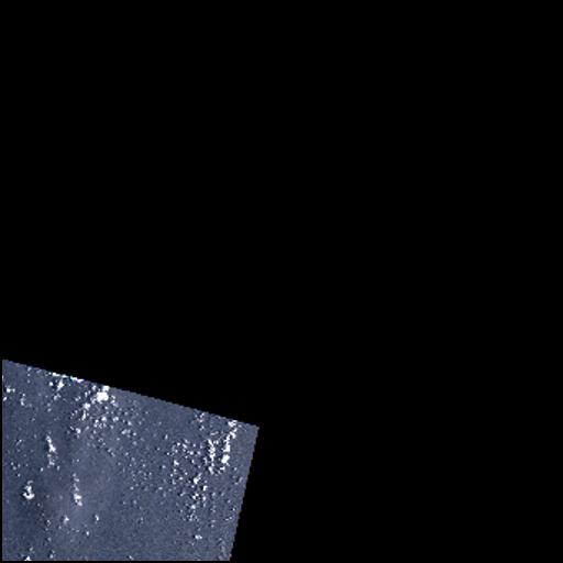
Now we can have a look at our items.
[25]:
for item in filtered["item"]:
    print(f"Quicklook of {item}")
    item.show_quicklook()
Quicklook of Item (URN:FEATURE:DATA:gdh:ccd73d19-4604-3d80-8bd6-88e4067cb916:V1)
/work/scratch/data/robertm/dev/env_tmp/pygeodes_cible/lib/python3.11/site-packages/urllib3/connectionpool.py:1097: InsecureRequestWarning: Unverified HTTPS request is being made to host 'geodes-portal.cnes.fr'. Adding certificate verification is strongly advised. See: https://urllib3.readthedocs.io/en/latest/advanced-usage.html#tls-warnings
  warnings.warn(
Downloading items#
Now we could want to download these items for further use :
[26]:
for item in filtered["item"]:
    item.download_archive()
/work/scratch/data/robertm/dev/env_tmp/pygeodes_cible/lib/python3.11/site-packages/urllib3/connectionpool.py:1097: InsecureRequestWarning: Unverified HTTPS request is being made to host 'geodes-portal.cnes.fr'. Adding certificate verification is strongly advised. See: https://urllib3.readthedocs.io/en/latest/advanced-usage.html#tls-warnings
  warnings.warn(
Download completed at /work/scratch/data/robertm/dev/pygeodes/docs/source/user_guide/S2C_MSIL1C_20260215T035841_N0512_R004_T48TTL_20260215T055156.zip
As we provided /tmp as default download dir, the downloads are stored in this folder.
[ ]: