Swot L2_LR_SSH

Swot L2_LR_SSH#

This chapter will present the functionalities specific to the Level 2 SWOT Low Rate products.

from fcollections.implementations import (
    # Handler
    NetcdfFilesDatabaseSwotLRL2,
    # Version
    L2Version, Timeliness)

import matplotlib.pyplot as plt
import matplotlib.patches as patches
import cartopy.crs as ccrs

Data samples#

We will illustrate the functionalities using a data sample from AVISO. You can use the altimetry-downloader-aviso tool to run the following script.

import logging
from pathlib import Path

from altimetry_downloader_aviso import get

logging.basicConfig()
logging.getLogger("altimetry_downloader_aviso").setLevel("INFO")

DATA_DIR = Path(__file__).resolve().parent.parent / "data"
DATA_DIR.mkdir(exist_ok=True)

if __name__ == "__main__":

    get(
        "SWOT_L2_LR_SSH_Basic",
        output_dir=DATA_DIR,
        cycle_number=[9, 10, 11],
        pass_number=[10, 11],
        version="P?C?",
    )

    get(
        "SWOT_L2_LR_SSH_Unsmoothed",
        output_dir=DATA_DIR,
        cycle_number=9,
        pass_number=10,
        version="PGC?",
    )

Query overview#

Detailed information on the filters and reading arguments can be found in the query API description

fcollections.implementations.NetcdfFilesDatabaseSwotLRL2.query()

The following examples can be used to build complex queries

Half Orbits

A unique half orbit

fc.query(cycle_number=1, pass_number=1)

One half orbit repeating over all cycles
```
fc.query(pass_number=1)
```

A list of half orbits, over multiple cycles

fc.query(cycle_number=slice(1, 4), pass_number=[1, 3])

Periods

A time stamp
```
fc.query(time='2024-01-01')
```

A period

fc.query(time=('2024-01-01', '2024-03-31'))

Variables subset

A subset of variables
```
fc.query(selected_variables=['time', 'longitude', 'latitude'])
```
Note

Available variables can explored using fcollections.implementations.NetcdfFilesDatabaseSwotLRL2.variables_info()

Area selection

Zoom over an area selection
```
fc.query(bbox=(-10, 5, 35, 40))
```

Reading options

Left swath (Unsmoothed only)

fc.query(left_swath=True, right_swath=False)

Right swath (Unsmoothed only)

fc.query(left_swath=False, right_swath=True)

Stacking over cycles (Basic, Expert, Windwave only)
```
fc.query(stack='CYCLES')
```
Stacking over both cycles and passes (Basic, Expert, Windwave only)
```
fc.query(stack='CYCLES_PASSES')
```

Subset definitions

Use baseline C versions
```
fc.query(version='P?C?')
```
Use a specific baseline, and only reprocessed data
```
fc.query(version='PGD?')
```
Complete version specification
```
fc.query(version='PGD0_02')
```
Choose one dataset
```
fc.query(subset='Expert')
```

Stack for temporal analysis#

The most prominent functionality is the ability to stack the half orbits when the grid is fixed (Basic, Expert and WindWave subsets). This allows to work along the cycle_number dimension and compute temporal analysis (mean, standard deviation, …).

There are currently three modes for stacking the half orbits

NOSTACK: do not stack the half orbits
CYCLES: concatenate the half orbits of one cycle along the num_lines dimension, and stack the cycles along a new cycle_number dimension
CYCLES_PASSES: stack the half orbits along the cycle_number and pass_number dimensions. Useful for regional analysis where the half orbits are cropped and we need an additional dimension to reflect the spatial jump

fc = NetcdfFilesDatabaseSwotLRL2("data")
ds = fc.query(stack='CYCLES', cycle_number=[9, 10, 11], pass_number=10, subset='Basic')
ds.ssha_karin_2.data

	Array	Chunk
Bytes	15.58 MiB	5.19 MiB
Shape	(3, 9866, 69)	(1, 9866, 69)
Dask graph	3 chunks in 10 graph layers
Data type	float64 numpy.ndarray

ds = fc.query(stack='CYCLES_PASSES', cycle_number=[9, 10, 11], pass_number=[10, 11], subset='Basic')
ds.ssha_karin_2.data

	Array	Chunk
Bytes	31.16 MiB	5.19 MiB
Shape	(2, 3, 9866, 69)	(1, 1, 9866, 69)
Dask graph	6 chunks in 23 graph layers
Data type	float64 numpy.ndarray

Note

Incomplete cycles are completed with invalids

Filter Level-2 version#

The Level-2 version is a complex tag composed of a temporality (forward I or reprocessed G), a baseline (major version A, B, C, D, …), a minor version (0, 1, 2, ..) and a product counter (01, 02, …). The fcollections.implementations.L2Version class can handle the tag information and filter out non-desired versions. It can be partially initialized in order to control the granularity of the filter.

version = L2Version(temporality=Timeliness.I)
version

PI??

fc.list_files(cycle_number=10, pass_number=10, version=version)

	cycle_number	pass_number	time	level	subset	version	filename
0	10	10	[2024-01-25T08:02:33.000000, 2024-01-25T08:54:...	ProductLevel.L2	ProductSubset.Basic	PIC0_01	/home/runner/work/fcollections/fcollections/do...

version = L2Version(baseline='C')
version

P?C?

fc.list_files(cycle_number=9, pass_number=10, version=version)

	cycle_number	pass_number	time	level	subset	version	filename
0	9	10	[2024-01-04T11:17:27.000000, 2024-01-04T12:08:...	ProductLevel.L2	ProductSubset.Basic	PGC0_01	/home/runner/work/fcollections/fcollections/do...
1	9	10	[2024-01-04T11:17:28.000000, 2024-01-04T12:08:...	ProductLevel.L2	ProductSubset.Unsmoothed	PGC0_01	/home/runner/work/fcollections/fcollections/do...
2	9	10	[2024-01-04T11:17:27.000000, 2024-01-04T12:08:...	ProductLevel.L2	ProductSubset.Basic	PIC0_01	/home/runner/work/fcollections/fcollections/do...

Area selection#

It is possible to select data crossing a specific region by providing bbox parameter to query or list_files method.

The bounding box is represented by a tuple of 4 float numbers, such as : (longitude_min, latitude_min, longitude_max, latitude_max). Its longitude must follow one of the known conventions: [0, 360[ or [-180, 180[.

If bbox’s longitude crosses -180/180, data around the crossing and matching the bbox will be selected. (e.g. for an interval [170, -170] -> both [170, 180[ and [-180, -170] intervals will be used to list/subset data).

To list files corresponding to half orbits crossing the bounding box:

bbox = -126, 32, -120, 40
fc.list_files(
    version='PIC?',
    subset='Basic',
    bbox=bbox)

	cycle_number	pass_number	time	level	subset	version	filename
0	9	11	[2024-01-04T12:08:54.000000, 2024-01-04T12:59:...	ProductLevel.L2	ProductSubset.Basic	PIC0_01	/home/runner/work/fcollections/fcollections/do...
1	11	11	[2024-02-15T05:39:04.000000, 2024-02-15T06:29:...	ProductLevel.L2	ProductSubset.Basic	PIC0_01	/home/runner/work/fcollections/fcollections/do...
2	10	11	[2024-01-25T08:54:00.000000, 2024-01-25T09:44:...	ProductLevel.L2	ProductSubset.Basic	PIC0_01	/home/runner/work/fcollections/fcollections/do...

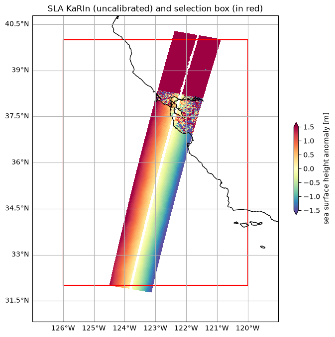
To query a subset of Swot LR L2 data crossing the bounding box:

Note

Lines of the swath crossing the bounding box will be entirely selected.

bbox = -126, 32, -120, 40
ds_area = fc.query(subset="Basic", version='P?C?', cycle_number=9, pass_number=11, bbox=bbox)

# Figure
localbox_cartopy = bbox[0] - 1, bbox[2] + 1, bbox[1] - 1, bbox[3] + 1
fig, ax = plt.subplots(figsize=(8, 8), subplot_kw=dict(projection=ccrs.PlateCarree()))
ax.set_extent(localbox_cartopy)

plot_kwargs = dict(
    x="longitude",
    y="latitude",
    cmap="Spectral_r",
    vmin=-1.5,
    vmax=1.5,
    cbar_kwargs={"shrink": 0.3},)

# SWOT KaRIn SLA plots
ds_area.ssha_karin_2.plot.pcolormesh(ax=ax, **plot_kwargs)
ax.set_title("SLA KaRIn (uncalibrated) and selection box (in red)")
ax.coastlines()
ax.gridlines(draw_labels=['left', 'bottom'])


# Add the patch to the Axes
rect = patches.Rectangle((bbox[0], bbox[1]), bbox[2] - bbox[0], bbox[3] - bbox[1], linewidth=1.5, edgecolor='r', facecolor='none')
ax.add_patch(rect)

<matplotlib.patches.Rectangle at 0x7efd8c880740>

../_images/2d5bf30567d8215e20648c45bbf9ce5be5d8a2a14b8d3d3ee01ddd4f0e7f99b5.png

Swath sides in Level-2 Unsmoothed subset#

The L2_LR_SSH Unsmoothed dataset files are using netcdf groups to separate the swath sides. This means we can open one of the two sides. The following figure illustrates how the left_swath and right_swath parameters can be used to retrieve one or the other side.

ds_left = fc.query(subset='Unsmoothed', cycle_number=9, pass_number=10, left_swath=True, right_swath=False,
                  selected_variables=['longitude', 'latitude', 'sig0_karin_2']).compute()
ds_right = fc.query(subset='Unsmoothed', cycle_number=9, pass_number=10, left_swath=False, right_swath=True,
                  selected_variables=['longitude', 'latitude', 'sig0_karin_2']).compute()


fig, (ax1, ax2) = plt.subplots(1, 2, figsize=(8, 4))

plot_kwargs = dict(
    cmap="Greys_r",
    cbar_kwargs={"shrink": 0.3},
    vmin=5, vmax=60)

# SWOT KaRIn SLA plots
s = slice(45000, 50000, 3)
ds_left.isel(num_lines=s).sig0_karin_2.plot.imshow(ax=ax1, **plot_kwargs)
ds_right.isel(num_lines=s).sig0_karin_2.plot.imshow(ax=ax2, **plot_kwargs)

ax1.set_title("Sigma0 KaRIn Left Swath")
ax2.set_title("Sigma0 KaRIn Right Swath")
fig.tight_layout()

../_images/3fb5cc9c7b9d55abb95750eba56acbefc33acc6fe7fba25b825c029d5041b661.png

Note

Combination of both sides is not yet possible. Moreover, keep in mind that position coordinates may include invalids which can break geo-plots.

Swot L2_LR_SSH

Contents

Swot L2_LR_SSH#

Data samples#

Query overview#

Stack for temporal analysis#

Filter Level-2 version#

Area selection#

Swath sides in Level-2 Unsmoothed subset#